Exploring K-Means clustering analysis in R Science 18.06.2016

Introduction: supervised and unsupervised learning

Machine learnin is one of the disciplines that is most frequently used in data mining and can be subdivided into two main tasks: supervised learning and unsupervised learning.

Supervised learning. This is a task of machine learning, which is executed by a set of methods aimed to infer a function from the training data. Normally, the training data is composed of a set of observations. Each observation possesses a diverse number of variables named predictors, and one variable that we want to predict, also known as labels or classes. These labels or classes represent the teachers because the models learn from them.

The ultimate aim of the function created by the model is the extrapolation of its behavior towards new observations, that is, prediction. This prediction corresponds to the output value of a supervised learning model that could be numeric, as in the case of a regression problem; or a class, as in the case of classification problems.

Below are some examples of supervised learning models

• Regression models
• Neural networks
• Support vector machines
• Random forests
• Boosting algorithms

The unsupervised learning is a machine learning task that aims to describe the associations and patterns in relation to a set of input variables. The fundamental difference from supervised learning is that input data has no class labels, so it has no variables to predict and rather tries to find data structures by their relationship.

In unsupervised learning, we can speak of two stages: modeling and profiting.

In the modeling phase, we take the input data and proceed to apply techniques of feature selection or feature extraction. Once we define the most convenient variables, we proceed to choose the best method of unsupervised learning to solve the problem at hand.

After choosing the method, we proceed to build the model and execute an iterative tuning process until we are satisfied with the results. In contrast to supervised learning, in which the model value is derived mostly from prediction, in unsupervised learning, the findings obtained during the modeling phase could be enough to fulfill the purpose, in which case, the process would stop. For example, if the objective is to make a customer group, once done, the modeling phase will have an idea of the existing groups, and that could be the goal of the analysis.

Assuming that the model was subsequently used, there is a second stage, which is when we have the model and want to exploit it again. We will receive new data and use the model that we built to run on them and get results.

Below are some examples of unsupervised learning models

• Clustering analysis
• Association rules

Preprocessing and standardization of data

Identifying groups (clustering analysis) can uncover and help to explain some patterns hiding in data and it is frequently the answer for multiple problems in many industries or contexts. Finding clusters can help to find relationships between study variables, but not the relations that these variables may have in relation to a target variable.

Typically, the application of clustering techniques involves five phases

1. Developing a working dataset.
2. Preprocessing and standardization of data.
3. Finding clusters in the data.
4. Interpreting those clusters, and finding conclusions.

In fact, when data is good, the construction of models that will respond to our problems becomes easier. Considering that clustering models work with distances, they are especially influenced by the data that we use.

Rescaling data. Whichever model we use will assume different things about the data. In the case of clustering models, it is very important that data, from the different numerical variables, expressed on a similar scale. When distances are calculated, if the units are very different, we cannot get proper results. For example, if we are doing an analysis related to a group of people and we have, among other data, the dollar income and age of the subjects, a variable such as income could overshadow the age variable. For analysis, 20 years of age may be more important than a $10,000 income. However, when compared both by measure of distances, a clustering model might underestimate the importance of age.

In order to mitigate the problem of the scale of the data, we can use methods of standardization. The standardization is the process of adjusting the data to a specific range, for example, between 0 and 1 or between –1 and 1.

There are several techniques for normalization

• recenter
• scale between 0 and 1
• median/MAD

The recenter performs a standard z-score transformation. The variable’s mean value is subtracted from each value and each one is then divided by the standard deviation. The resulting variable will have a mean of 0 and a standard deviation of 1.

After transformation, the variables are not expressed in their original scales, for example, age no longer displays a number of years. To make it interesting while performing a test, we can confirm that the transformation does not affect the relationship between the variables:

ages = sample(12:100, 20, replace=T)
incomes = sample(500:10000, 20, replace=T)
data = cbind(ages, incomes)
scaled = scale(data)

# comparing correlations    
# data before transformation    
cor(data)

# data after transformation
cor(scaled)

Another method for make transformation is the Scale [0-1]: just rescale the original values into the 0 - 1 range. This is done by subtracting the minimum value from the variable’s value for each observation and, then, dividing by the difference between the minimum and the maximum values.

If we want to implement this transformation method, we can use the reshape package, in particular the rescaler function

# install.packages("reshape")
library("reshape")

scaled = rescaler(data, "range")
head(scaled)

Median/MAD is a robust version of the standard recenter transform. The median value is subtracted from each value, and each is then divided by the median absolute deviation. The resulting variable will have a median of 0.

The function is included in the reshape package and its use is very similar to the previous example

# install.packages("reshape")
library("reshape")

scaled = rescaler(data, "robust")
head(scaled)

Clustering analysis

Clustering is based on the concepts of similarity and distance, while proximity is determined by a distance function. It allows the generation of clusters where each of these groups consists of individuals who have common features with each other.

Clustering is used for knowledge discovery rather than prediction. It provides an insight into the natural groupings found within data.

The analysis of clusters is similar to the classification models, with the difference that the groups are not preset (labels). The goal is to perform a partition of data into clusters that can be disjoint or not.

Clustering model is a notion used to signify what kind of clusters we are trying to identify. The four most common models of clustering methods are hierarchical clustering, k-means clustering, model-based clustering, and density-based clustering:

• Hierarchical clustering. It creates a hierarchy of clusters, and presents the hierarchy in a dendrogram. This method does not require the number of clusters to be specified at the beginning. Distance connectivity between observations is the measure.
• k-means clustering. It is also referred to as flat clustering. Unlike hierarchical clustering, it does not create a hierarchy of clusters, and it requires the number of clusters as an input. However, its performance is faster than hierarchical clustering. Distance from mean value of each observation/cluster is the measure.
• Model-based clustering (or Distribution models). Both hierarchical clustering and k-means clustering use a heuristic approach to construct clusters, and do not rely on a formal model. Model-based clustering assumes a data model and applies an EM algorithm to find the most likely model components and the number of clusters. Significance of statistical distribution of variables in the dataset is the measure.
• Density-based clustering. It constructs clusters in regard to the density measurement. Clusters in this method have a higher density than the remainder of the dataset. Density in data space is the measure.

A good clustering algorithm can be evaluated based on two primary objectives:

• High intra-class similarity
• Low inter-class similarity

Clustering tendency

Most clustering algorithms will always produce a clustering, even if the data does not contain a cluster structure. It is typically good to check cluster tendency before attempting to cluster the data.

Prepare data for iris dataset.

#install.packages("seriation")
library(seriation)

d_iris <- dist(iris[,-5])

Visual Analysis for Cluster Tendency Assessment (VAT) reorders the objects to show potential clustering tendency as a block structure (dark blocks along the main diagonal).

VAT(d_iris)

iVAT uses largest distances in all possible paths between the objects instead of the distances to make the block structure better visible.

iVAT(d_iris)

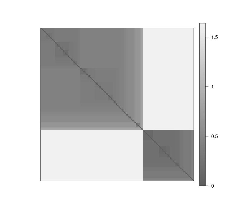
Both plots show a strong cluster structure with 2 clusters.

K-Means algorithm

There are many methods, and the most popular are based on Hierarchical Classification and dynamic clouds or K-Means.

In very general terms, the K-Means algorithm aims to partition a set of observations into k clusters so that each observation belongs to the cluster that possesses the nearest mean. It just finds the k different groups that have the maximum dissimilarity.

Since the mean is used as a measure of estimating the centroid, it is not free from the presence of extreme observations or outliers. Hence, it is required to check the presence of outliers in a dataset before running k-means clustering. We can the boxplot method of identifying the presence of any outliers in the our dataset.

You can see video How K-Means algorithm works or K-means Algorithm Demo.

Main features of K-Means algorithm:

• proper for compact clusters
• sensitive to outliers and noise
• uses only numerical attributes

In the simplest form of the algorithm, it has two steps:

• Assignment. Assign each observation to the cluster that gives the minimum within cluster sum of squares (WCSS).
• Update. Update the centroid by taking the mean of all the observation in the cluster.

These two steps are iteratively executed until the assignments in any two consecutive iteration don’t change, meaning either a point of local or global optima (not always guaranteed) is reached.

All steps of K-Means algorithm:

1. Select K points as initial centroids.
2. repeat
3.    Form K clusters by assigning each point to its closest centroid.
4.    Recompute the centroid of each cluster.
5. until Centroids do not change.

Although it is a computationally difficult problem, there are very efficient implementations to quickly find the local optimum. In an optimization problem, the optimum is the value that maximizes or minimizes the condition that we are looking for.

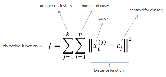
Given a set of observations , K-Means clustering aims to partition the N observations into sets so as to minimize the within-cluster sum of squares (WCSS):

The method of Forgy and Random partition are the most common initialization approaches. Forgy chooses k observations from the data and uses these as the initial means. The method first assigns a cluster to each observation at random, then proceeds to the update phase, thereby computing the initial mean to become the centroid of the cluster’s randomly assigned points. The assignment phase is also referred to as the expectation phase, and the update phase as the maximization phase, making this algorithm a variant of the generalized expectation maximization algorithm.

In R, there are several packages that allow us to use K-Means. The following is an implementation using the Iris dataset

# build the K-Means standard model
set.seed(42)
k = 3
km = kmeans(iris[1:4], k, iter.max=1000, algorithm=c("Forgy"))

The K-Means function requires that we properly define two important parameters: the number of clusters that it is convenient to use and the type of the function algorithm to be used to establish the optimum.

We can see some information about the outcome

# size of clusters
km$size
[1] 62  38  50

# centers of clusters, three clusters by variable
km$centers

Based on the numerical data of Iris, model K-Means builds three groups, as we indicated, and then proceeds to classify each observation, in one of those groups.

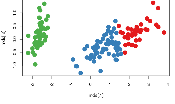
Let's plot the result. This allows for a better appreciation of the information, so we must reduce the dataset to be represented in two dimensions

# translate into a two dimensions using multidimensional scaling
dist = dist(iris[1:4])
mds = cmdscale(dist)

palette(c("#E41A1C", "#377EB8", "#4DAF4A", "#984EA3",  "#FF7F00", "#FFFF33", "#A65628", "#F781BF", "#999999", "#000000"))
plot(mds, col=km$cluster, pch = 20, cex = 3)

# plot centroids
km1 = kmeans(mds, k, iter.max=1000, algorithm=c("Forgy"))
points(km1$centers, col = 10, pch = 8, cex = 2)

You can draw the centers of each cluster in a barplot, which will provide more details on how each attribute affects the clustering. To inspect the center of each cluster input following command.

barplot(t(km$centers), beside=TRUE, xlab="cluster", ylab="value")

install.packages("cluster")
library("cluster")

# cluster plot 
clusplot(mds, km$cluster, color=TRUE, shade=TRUE, labels=2, lines=1, main='Cluster Analysis for Iris')

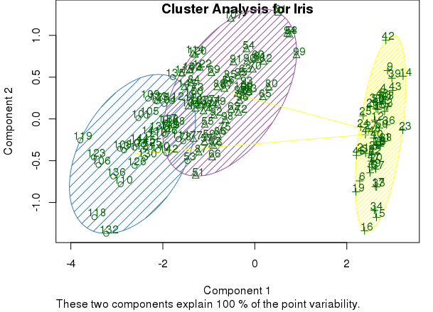
The graphic expression of clusters can help to evaluate whether the result makes sense. If we determine that it does, we can also include the results of cluster analysis in the original dataset. Then we can work on R or also export it to other tools

# add cluster to original dataset
iris.cluster = cbind(iris, km[1])

head(iris.cluster[3:6])

Let us compare the clusters with the species

table(km$cluster, iris$Species)

Using the aggregate() function, we can also look at the Sepal.Length characteristics of the clusters. aggregate() function computes statistics for subgroups of data. Here, it calculates the mean Sepal.Length by cluster:

aggregate(data = iris.cluster, Sepal.Length ~ cluster, mean)

Other approaches for clustering

Partitioning Around Medoids (PAM) is similar to K-Means, but it is more robust with outliers. It can be implemented using pam() from cluster package.

#install.packages("cluster")
library("cluster")
# implements PAM function
cls = pam(iris[1:4], 3)  
# display cluster plot an silhouette plot
plot(cls) 
# display cluster diagnostics
summary(cls) 

The summary(cls) calculated above from pam() gives the silhouette width information for each data point. Silhouette width is a measure to estimate the dissimilarity between clusters. A higher silhouette width is preferred to determine the optimal number of clusters.

Clustering Large Applications (CLARA) is useful for clustering large datasets. clara() from cluster package uses a sampling approach to cluster large datasets. It provide silhouette plot and information to determine optimum number of clusters.

#install.packages("cluster")
library("cluster")

# cluster with clara
cls = clara (iris[1:4], 3, samples=50) 
summary(cls)
plot(cls)

Defining the number of clusters

As the k-means algorithm is highly sensitive to the starting position of the cluster centers, this means that random chance may have a substantial impact on the final set of clusters. The choice requires a delicate balance.

There are different methods for determining the optimal number of clusters for k-means. These methods include direct methods and statistical testing methods. You can read more here.

• Direct methods consists of optimizing a criterion, such as the within cluster sums of squares or the average silhouette. The corresponding methods are named elbow and silhouette methods, respectively.
• Testing methods consists of comparing evidence against null hypothesis. An example is the gap statistic.

There are several tips how to choose the appropriate number of clusters:

• Ideally, you will have a priori knowledge about the true groupings and you can apply this information to choosing the number of clusters.
• Sometimes the number of clusters is dictated by business requirements or the motivation for the analysis.
• Without any prior knowledge, one rule of thumb suggests setting k equal to the square root of (n / 2), where n is the number of examples in the dataset. However, this rule of thumb is likely to result in an unwieldy number of clusters for large datasets.
• There are numerous statistics to measure homogeneity and heterogeneity within the clusters that can be used.

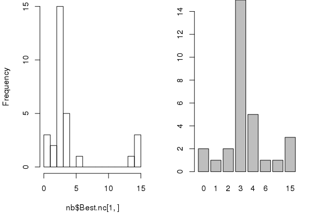
NbClust package. The NbClust package provides 30 indices for determining the number of clusters and proposes to the user the best clustering scheme from the different results obtained by varying all combinations of number of clusters, distance measures, and clustering methods.

In the following snippet we find the suggested amount of clusters

install.packages("NbClust")
library("NbClust")

data = iris[,-5]

nb = NbClust(data, diss=NULL, distance="euclidean", min.nc=2, max.nc=15, method="complete", index="alllong")

The package also has some graphical indices.

# sets 1x2 grid for plotting
par(mfrow=c(1, 2))

# making graph of recounts
hist(nb$Best.nc[1,], breaks=max(na.omit(nb$Best.nc[1,])))
barplot(table(nb$Best.nc[1,]))

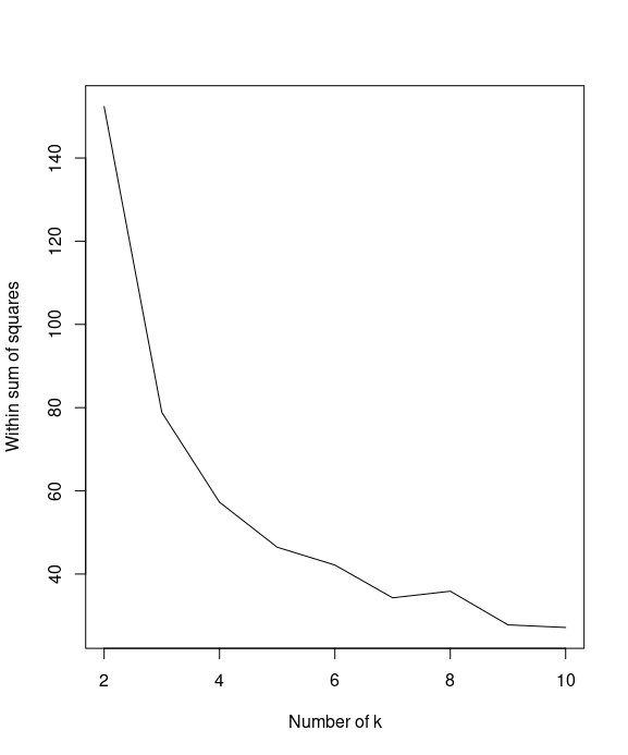
Sum of squares. Also, we can use the sum of squares to determine which k value is best for finding the optimum number of clusters for k-means.

We'll demonstrate how to find the optimum number of clusters by iteratively getting within the sum of squares and the average silhouette value. For the within sum of squares, lower values represent clusters with better quality. Perform the following steps to find the optimum number of clusters for the k-means clustering.

First, calculate the within sum of squares (withinss) of different numbers of clusters:

k = 2:10
set.seed(42)
WSS = sapply(k, function(k) {kmeans(iris[1:4], centers=k)$tot.withinss})

You can then use a line plot to plot the within sum of squares with a different number of k

plot(k, WSS, type="l", xlab= "Number of k", ylab="Within sum of squares")

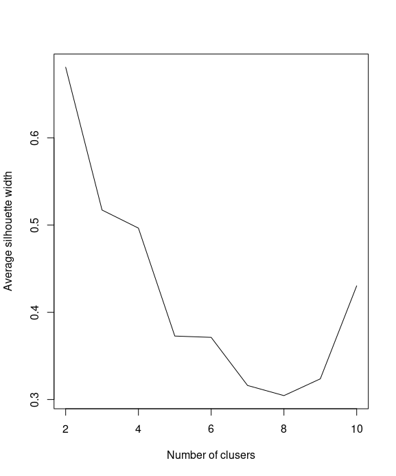
Next, you can calculate the average silhouette width (avg.silwidth) of different numbers of clusters

SW = sapply(k, function(k) {cluster.stats(dist(iris[1:4]), kmeans(iris[1:4], centers=k)$cluster)$avg.silwidth})

You can then use a line plot to plot the average silhouette width with a different number of k

plot(k, SW, type="l", xlab="Number of clusers", ylab="Average silhouette width")

By plotting the within sum of squares in regard to different number of k, we find that the elbow of the plot is at k=2.

We use which.max to obtain the value of k to determine the location of the maximum average silhouette width and retrieve the maximum number of clusters:

k[which.max(SW)]

gap statistic. Alternative approach is gap statistic. The approach can be applied to any clustering method (K-means clustering, hierarchical clustering, etc).

The gap statistic compares the total within intracluster variation for different values of k with their expected values under null reference distribution of the data, i.e. a distribution with no obvious clustering.

library("factoextra")
fviz_nbclust(iris[,-5], kmeans, method = "gap_stat")

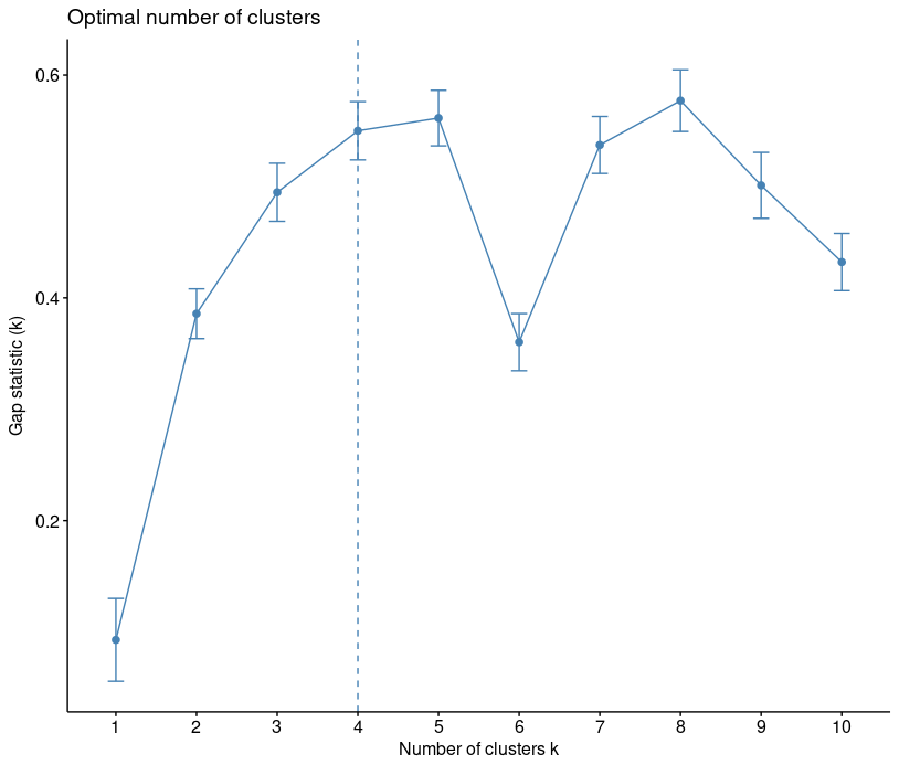
You can see that recommended choice of clusters is 4.

Evaluation of clustering

Internal Evaluation. When a clustering result is evaluated based on the data that was clustered, it is called internal evaluation. These methods usually assign the best score to the algorithm that produces clusters with high similarity within a cluster and low similarity between clusters. There are following methods for internal evaluation:

• Dunn Index
• Silhouette Coefficient

External Evaluation. External evaluation is similar to evaluation done on test data. The data used for testing is not used for training the model. The test data is then evaluated and labels assigned by experts or some third party benchmarks. Then clustering results on these already labeled items provide us the metric for how good the clusters grouped our data. As the metric depends on external inputs, it is called external evaluation. There are following methods for External evaluation:

• Rand Measure
• Jaccard Index

Outcome

K-means clustering is an unsupervised learning algorithm that tries to combine similar objects into a group in such a way that the within-group similarity should be maximum and the between-group object similarity should be minimum.

The algorithm's goal is to minimize the within-cluster variation as defined by the squared Euclidean distances.

Merits of K-means clustering:

• It is simple to understand and easy to interpret
• It is more flexible in comparison to other clustering algorithms
• Performs well on a large number of input features

Demerits of K-means clustering:

• It is not based on robust methodology. The big problem is initial random points
• Different random points display different results. Hence, more iteration is required.
• Since more iteration is required, it may not be efficient for large datasets from a computational efficiency point of view. It would require more memory to process.
• Computed local optimum is known to be a far cry from the global one.
• It is not obvious what is a good k to use.
• The process is sensitive with respect to outliers.
• The algorithm lacks scalability.
• Only numerical attributes are covered.
• Resulting clusters can be unbalanced (in Forgy’s version, even empty).

Useful book

• Unsupervised Learning with R