Exploring Hierarchical clustering in R Science 29.01.2017

Introduction

Clustering is a multivariate analysis used to group similar objects (close in terms of distance) together in the same group (cluster). Unlike supervised learning methods (for example, classification and regression) a clustering analysis does not use any label information, but simply uses the similarity between data features to group them into clusters.

Clustering does not refer to specific algorithms but it’s a process to create groups based on similarity measure. Clustering analysis use unsupervised learning algorithm to create clusters.

Clustering algorithms generally work on simple principle of maximization of intracluster similarities and minimization of intercluster similarities. The measure of similarity determines how the clusters need to be formed.

Similarity is a characterization of the ratio of the number of attributes two objects share in common compared to the total list of attributes between them. Objects which have everything in common are identical, and have a similarity of 1.0. Objects which have nothing in common have a similarity of 0.0.

Clustering can be widely adapted in the analysis of businesses. For example, a marketing department can use clustering to segment customers by personal attributes. As a result of this, different marketing campaigns targeting various types of customers can be designed.

Clustering model is a notion used to signify what kind of clusters we are trying to identify. The four most common models of clustering methods are hierarchical clustering, k-means clustering, model-based clustering, and density-based clustering:

• Hierarchical clustering. It creates a hierarchy of clusters, and presents the hierarchy in a dendrogram. This method does not require the number of clusters to be specified at the beginning. Distance connectivity between observations is the measure.
• k-means clustering. It is also referred to as flat clustering. Unlike hierarchical clustering, it does not create a hierarchy of clusters, and it requires the number of clusters as an input. However, its performance is faster than hierarchical clustering. Distance from mean value of each observation/cluster is the measure.
• Model-based clustering (or Distribution models). Both hierarchical clustering and k-means clustering use a heuristic approach to construct clusters, and do not rely on a formal model. Model-based clustering assumes a data model and applies an EM algorithm to find the most likely model components and the number of clusters. Significance of statistical distribution of variables in the dataset is the measure.
• Density-based clustering. It constructs clusters in regard to the density measurement. Clusters in this method have a higher density than the remainder of the dataset. Density in data space is the measure.

A good clustering algorithm can be evaluated based on two primary objectives:

• High intra-class similarity
• Low inter-class similarity

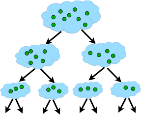
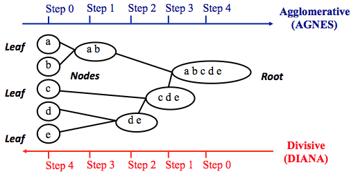
Hierarchical clustering adopts either an agglomerative or divisive method to build a hierarchy of clusters. Regardless of which approach is adopted, both first use a distance similarity measure to combine or split clusters. The recursive process continues until there is only one cluster left or you cannot split more clusters. Eventually, we can use a dendrogram to represent the hierarchy of clusters.

• Agglomerative hierarchical clustering. This is a bottom-up approach. Each observation starts in its own cluster. We can then compute the similarity (or the distance) between each cluster and then merge the two most similar ones at each iteration until there is only one cluster left.
• Divisive hierarchical clustering. This is a top-down approach. All observations start in one cluster, and then we split the cluster into the two least dissimilar clusters recursively until there is one cluster for each observation.

The agglomerative methods, using a recursive algorithm that follows the next phases:

• Find the two closest points in the dataset.
• Link these points and consider them as a single point.
• The process starts again, now using the new dataset that contains the new point.

In a hierarchical clustering, there are two very important parameters: the distance metric and the linkage method.

Clustering distance metric. Defining closeness is a fundamental aspect. A measure of dissimilarity is that which defines clusters that will be combined in the case of agglomerative method, or that, in the case of divisive clustering method, when these are to be divided. The main measures of distance are as follows:

• Euclidean distance
• Maximum distance
• Manhattan distance
• Canberra distance
• Binary distance
• Pearson distance
• Correlation
• Spearman distance

You can read more about distance measure and it visualization here.

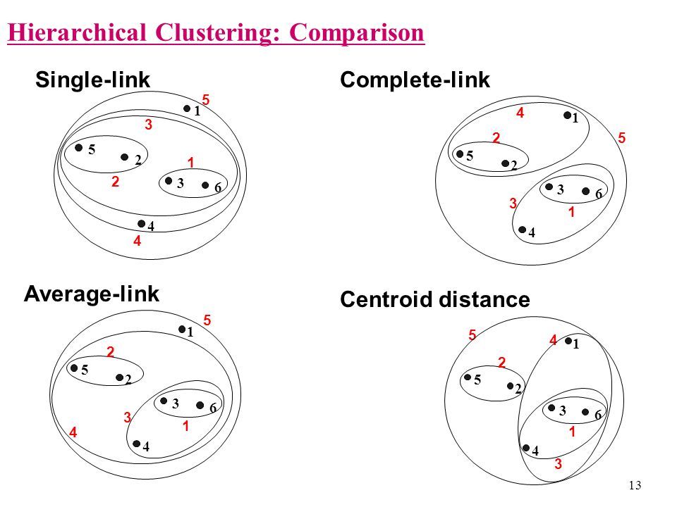
Linkage methods. The linkage methods determine how the distance between two clusters is defined. A linkage rule is necessary for calculating the inter-cluster distances. It is important to try several linkage methods to compare their results. Depending on the dataset, some methods may work better. The following is a list of the most common linkage methods:

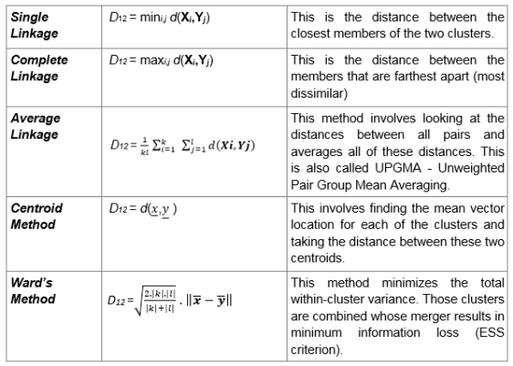
• Single linkage. This refers to the shortest distance between two points in each cluster. The distance between two clusters is the minimum distance between an observation in one cluster and an observation in the other cluster. A good choice when clusters are obviously separated.
• Complete linkage. This refers to the longest distance between two points in each cluster. The distance between two clusters is the maximum distance between an observation in one cluster and an observation in the other cluster. It can be sensitive to outliers.
• Average linkage This refer to the average distance between two points in each cluster. The distance between two clusters is the mean distance between an observation in one cluster and an observation in the other cluster.
• Ward linkage. This refers to the sum of the squared distance from each point to the mean of the merged clusters. The distance between two clusters is the sum of the squared deviations from points to centroids. Try to minimize the within-cluster sum of squares. It can be sensitive to outliers.
• Centroid Linkage. The distance between two clusters is the distance between the cluster centroids or means.
• Median Linkage. The distance between two clusters is the median distance between an observation in one cluster and an observation in the other cluster. It reduces the effect of outliers.
• McQuitty Linkage When two clusters A and B are be joined, the distance to new cluster C is the average of distances of A and B to C. So, the distance depends on a combination of clusters instead of individual observations in the clusters.

Hierarchical clustering is based on the distance connectivity between observations of clusters. The steps involved in the clustering process are:

1. Start with N clusters, N is number of elements (i.e., assign each element to its own cluster). In other words distances (similarities) between the clusters are equal to the distances (similarities) between the items they contain.
2. Now merge pairs of clusters with the closest to other (most similar clusters) (e.g., the first iteration will reduce the number of clusters to N - 1).
3. Again compute the distance (similarities) and merge with closest one.
4. Repeat Steps 2 and 3 to exhaust the items until you get all data points in one cluster.

Modeling in R

In R, we use the hclust() function for hierarchical cluster analysis. This is part of the stats package. To perform hierarchical clustering, the input data has to be in a distance matrix form.

Another important function used here is dist() this function computes and returns the distance matrix computed by using the specified distance measure to compute the distances between the rows of a data matrix. By default, it is Euclidean distance.

You can then examine the iris dataset structure:

str(iris)

Let's look at the parallel coordinates plot of the data.

Parallel coordinates are a common way of visualizing high-dimensional geometry and analyzing multivariate data. The lines show the relationship between the axes, much like scatterplots, and the patterns that the lines form indicate the relationship. You can also gather details about the relationships between the axes when you see the clustering of lines.

# get nice colors
library(colorspace)

iris2 <- iris[,-5]
species_labels <- iris[,5]
species_col <- rev(rainbow_hcl(3))[as.numeric(species_labels)]
MASS::parcoord(iris2, col = species_col, var.label = TRUE, lwd = 2)
title("Parallel coordinates plot of the Iris data")
legend("top", cex = 1, legend = as.character(levels(species_labels)), fill = unique(species_col), horiz = TRUE)

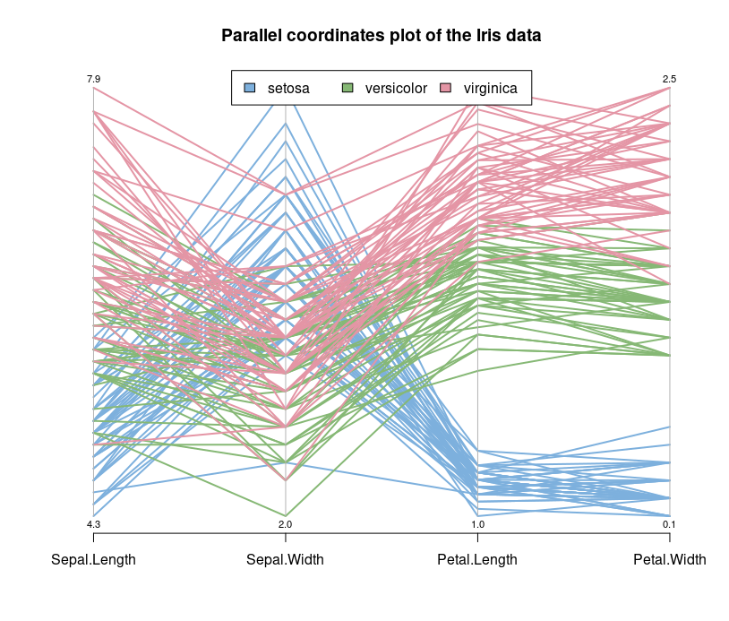
We can see that the Setosa species are distinctly different from Versicolor and Virginica (they have lower petal length and width). But Versicolor and Virginica cannot easily be separated based on measurements of their sepal and petal width/length.

You can then use agglomerative hierarchical clustering to cluster the customer data:

iris_hc = hclust(dist(iris[,1:4], method="euclidean"), method="ward.D2")

We use the Euclidean distance as distance metrics, and use Ward's minimum variance method to perform agglomerative clustering.

Lastly, you can use the plot function to plot the dendrogram:

plot(iris_hc, hang = -0.01, cex = 0.7)

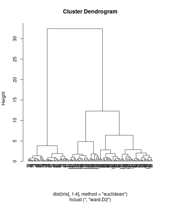
Finally, we use the plot function to plot the dendrogram of hierarchical clusters. We specify hang to display labels at the bottom of the dendrogram, and use cex to shrink the label to 70 percent of the normal size.

In the dendrogram displayed above, each leaf corresponds to one observation. As we move up the tree, observations that are similar to each other are combined into branches. You can see more kinds of visualizing dendrograms in R here or here.

In a dendrogram, we can see the hierarchy of clusters, but we have not grouped data into different clusters yet. However, we can determine how many clusters are within the dendrogram and cut the dendrogram at a certain tree height to separate the data into different groups. We'll demonstrate how to use the cutree function to separate the data into a given number of clusters.

First, categorize the data into four groups:

fit = cutree(iris_hc, k = 3)

You can then examine the cluster labels for the data:

fit

Count the number of data within each cluster:

table(fit, iris$Species)

Finally, you can visualize how data is clustered with the red rectangle border:

plot(iris_hc, hang = -0.01, cex = 0.7)
rect.hclust(iris_hc, k=3, border="red")
# rect.hclust(res.hc, k = 3, border = 2:4)

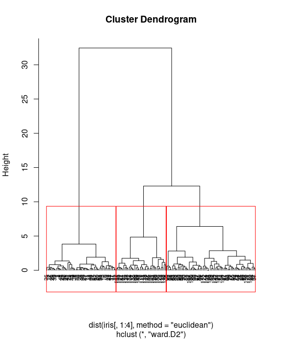
table the clustering distribution with actual Species

table(fit, iris$Species)

An alternative way to produce dendrograms is to specifically convert hclust objects into dendrograms objects.

# Convert hclust into a dendrogram and plot
hcd <- as.dendrogram(iris_hc)

# Default plot
plot(hcd, type = "rectangle", ylab = "Y")

# Define nodePar
nodePar <- list(lab.cex = 0.6, pch = c(NA, 19), 
    cex = 0.7, col = "blue")

# Customized plot; remove labels
plot(hcd, ylab = "Y", nodePar = nodePar, leaflab = "none")

# Horizontal plot
plot(hcd,  xlab = "Y",
    nodePar = nodePar, horiz = TRUE)

# Change edge color
plot(hcd,  xlab = "Height", nodePar = nodePar, 
    edgePar = list(col = 2:3, lwd = 2:1))     

The R package ggplot2 have no functions to plot dendrograms. However, the ad-hoc package ggdendro offers a decent solution.

# install.packages('ggdendro')
library(ggplot2)
library(ggdendro)

# basic option
ggdendrogram(iris_hc)

# another option
ggdendrogram(iris_hc, rotate = TRUE, size = 4, theme_dendro = FALSE, color = "tomato")

Using the function fviz_cluster() in factoextra], we can also visualize the result in a scatter plot. Observations are represented by points in the plot, using principal components. A frame is drawn around each cluster.

# install.packages('factoextra')
library(factoextra)
fviz_cluster(list(data=iris[,1:4], cluster=fit))

Comparing clustering methods

After fitting data into clusters using different clustering methods, you may wish to measure the accuracy of the clustering. In most cases, you can use either intracluster or intercluster metrics as measurements. The higher the intercluster distance, the better it is, and the lower the intracluster distance, the better it is.

We now introduce how to compare different clustering methods using cluster.stat from the fpc package.

Perform the following steps to compare clustering methods.

First, install and load the fpc package

#install.packages("fpc")
library("fpc")

You then need to use hierarchical clustering with the single method to cluster customer data and generate the object hc_single

single_c = hclust(dist(iris[,1:4]), method="single")
hc_single = cutree(single_c, k=3)

Use hierarchical clustering with the complete method to cluster customer data and generate the object hc_complete

complete_c = hclust(dist(iris[,1:4]), method="complete")
hc_complete = cutree(complete_c, k=3)

You can then use k-means clustering to cluster customer data and generate the object km

set.seed(1234)
km = kmeans(iris[1:4], 3, iter.max=1000, algorithm=c("Forgy"))

Next, retrieve the cluster validation statistics of either clustering method:

cs = cluster.stats(dist(iris[1:4]), km$cluster)

Most often, we focus on using within.cluster.ss and avg.silwidth to validate the clustering method. The within.cluster.ss measurement stands for the within clusters sum of squares, and avg.silwidth represents the average silhouette width.

• within.cluster.ss measurement shows how closely related objects are in clusters; the smaller the value, the more closely related objects are within the cluster.
• avg.silwidth is a measurement that considers how closely related objects are within the cluster and how clusters are separated from each other. The silhouette value usually ranges from 0 to 1; a value closer to 1 suggests the data is better clustered.

cs[c("within.cluster.ss","avg.silwidth")]

Finally, we can generate the cluster statistics of each clustering method and list them in a table:

sapply(list(kmeans = km$cluster, hc_single = hc_single, hc_complete = hc_complete),
    function(c) cluster.stats(dist(iris[1:4]), c)[c("within.cluster.ss","avg.silwidth")])

Data preparation

Remove any missing value (i.e, NA values for not available)

df <- na.omit(iris[,1:4])

Next, we have to scale all the numeric variables. Scaling means each variable will now have mean zero and standard deviation one. Ideally, you want a unit in each coordinate to represent the same degree of difference. Scaling makes the standard deviation the unit of measurement in each coordinate. This is done to avoid the clustering algorithm to depend to an arbitrary variable unit. You can scale/standardize the data using the R function scale:

data <- scale(df)

Useful links

• Hierarchical Clustering Essentials