Introduction to linear regression and modeling in R Science 06.06.2016

Introduction

In statistics, modeling is where we get down to business. Models quantify the relationships between our variables and one let us make predictions.

The regression analysis focus on building a thought process around how the modeling techniques establish and quantify a relation among response variables and predictors. Regression is to build a function of independent variables (also known as features, attributes, predictors, dimensions) to predict a dependent variable (also called response, output, target).

The concept of causation is important to keep in mind, as most of the time our thought process deviates from how relationships quantified by a model have to be interpreted. For example, a statistical model will be able to quantify relationships between completely irrelevant measures, say electricity generation and beer consumption.

Any regression analysis involves three key sets of variables:

• Dependent or response variables (Y): Input series
• Independent or predictor variables (X): Input series
• Model parameters: Unknown parameters to be estimated by the regression model

Important concept to understand is around parametric and non-parametric methods.

• Parametric methods assume that the sample data is drawn from a known probability distribution based on fixed set of parameters. For instance, linear regression assumes normal distribution, whereas logistic assumes binomial distribution, etc. This assumption allows the methods to be applied to small datasets as well.
• Non-parametric methods do not assume any probability distribution in prior, rather they construct empirical distributions from the underlying data. These methods require high volume of data to model estimation. There exists a separate branch on non-parametric regressions, e.g., kernel regression, Nonparametric Multiplicative Regression (NPMR) etc.

A simple linear regression is the most basic model. The linear regression model is used for explaining the relationship between a single dependent variable known as Y and one or more X's independent variables known as input, predictor, or independent variables. So, it’s just two variables and is modeled as a linear relationship with an error term

We are given the data for x and y. Our mission is to fit the model, which will give us the best estimates for and .

In other words, simple linear regression fits a straight line through the set of n points in such a way that makes the sum of squared residuals of the model (that is, vertical distances between the points of the data set and the fitted line) as small as possible.

That generalizes naturally to multiple linear regression, where we have multiple variables on the righthand side of the relationship

Statisticians call u, v, and w the predictors and y the response. Obviously, the model is useful only if there is a fairly linear relationship between the predictors and the response, but that requirement is much less restrictive than you might think.

The beauty of R is that anyone can build these linear models. The models are built by a function, lm , which returns a model object. From the model object, we get the coefficients () and regression statistics.

Regression creates a model, and ANOVA (Analysis of variance) is one method of evaluating such models. ANOVA is actually a family of techniques that are connected by a common mathematical analysis.

• One-way ANOVA. This is the simplest application of ANOVA. Suppose you have data samples from several populations and are wondering whether the populations have different means. One-way ANOVA answers that question. If the populations have normal distributions, use the oneway.test function, otherwise, use the nonparametric version, the kruskal.test function.
• Model comparison. When you add or delete a predictor variable from a linear regression, you want to know whether that change did or did not improve the model. The anova function compares two regression models and reports whether they are significantly different.
• ANOVA table. The anova function can also construct the ANOVA table of a linear regression model, which includes the F statistic needed to gauge the model’s statistical significance.

Essentially, the linear regression model will help you with:

• Prediction or forecasting
• Quantifying the relationship among variables

Simple linear regression

Imagine, you have two vectors, x and y, that hold paired observations: . You believe there is a linear relationship between x and y, and you want to create a regression model of the relationship.

The regression uses the ordinary least-squares (OLS) algorithm to fit the linear model

where and are the regression coefficients and the are the error terms.

The lm function can perform linear regression. The main argument is a model formula, such as y ~ x. The formula has the response variable on the left of the tilde character ( ~ ) and the predictor variable on the right. The function estimates the regression coefficients, and , and reports them as the intercept and the coefficient of x, respectively

lm(iris$Sepal.Length ~ iris$Sepal.Width)

In this case, the regression equation

iris$Sepal.Length = 6.5262 - 0.2234 iris$Sepal.Width

Multiple linear regression

Suppose you have several predictor variables (e.g., u, v, and w) and a response variable y. You believe there is a linear relationship between the predictors and the response, and you want to perform a linear regression on the data.

Multiple linear regression is the obvious generalization of simple linear regression. It allows multiple predictor variables instead of one predictor variable and still uses OLS to compute the coefficients of a linear equation. The three-variable regression just given corresponds to this linear model:

R uses the lm function for both simple and multiple linear regression. You simply add more variables to the righthand side of the model formula. The output then shows the coefficients of the fitted model:

lm(y ~ u + v + w)

Let's look at strengths and weaknesses of multiple linear regression.

Strength of multiple linear regression:

• By far the most common approach for modeling numeric data
• Can be adapted to model almost any modeling task
• Provides estimates of both the strength and size of the relationships among features and the outcome

Weaknesses of multiple linear regression:

• Makes strong assumptions about the data
• The model's form must be specified by the user in advance
• Does not handle missing data
• Only works with numeric features, so categorical data requires extra processing
• Requires some knowledge of statistics to understand the model

Getting regression statistics

Before interpreting and using your model, you will need to determine whether it is a good fit to the data and includes a good combination of explanatory variables. You may also be considering several alternative models for your data and want to compare them.

The fit of a model is commonly measured in a few different ways. These include:

• Coefficient of determination () gives an indication of how well the model is likely to predict future observations. It measures the portion of the total variation in the data that the model is able to explain. It takes values between 0 and 1. A value close to 1 suggests that the model will give good predictions, while a value close to 0 suggests that the model will make poor predictions.
• Significance test for model coefficients tells you whether individual coefficient estimates are significantly different from 0, and hence whether the coefficients are contributing to the model. Consider removing coefficients with p-values greater than 0.05.
• F-test tells you whether the model is significantly better at predicting compared with using the overall mean value as a prediction. For good models, the p-value will be less than 0.05. An F-test can also be used to compare two models. In this case, a p-value less than 0.05 tells you that the more complex model is significantly better than the simpler model.
• Confidence intervals for the coefficients.
• Residuals are the set of differences between the observed values of the response variable, and the values predicted by the model (the fitted values). Standardized residuals and studentized residuals are types of residuals that have been adjusted to have a variance of one.
• The ANOVA table.

Save the regression model in a variable, say m

m = lm(y ~ u + v + w)

Then use functions to extract regression statistics and information from the model

• anova(m) ANOVA table
• coefficients(m) Model coefficients
• coef(m) Same as coefficients(m)
• confint(m) Confidence intervals for the regression coefficients
• deviance(m) Residual sum of squares
• effects(m) Vector of orthogonal effects
• fitted(m) Vector of fitted y values
• residuals(m) Model residuals
• resid(m) Same as residuals(m)
• summary(m) Key statistics, such as , the F statistic, and the residual standard error (). You can read good description of summary in book "R Cookbook" by Paul Teetor (page 270).
• vcov(m) Variance–covariance matrix of the main parameters

Plotting regression residuals

Residuals are core to the diagnostic of regression models. Normality of residual is an important condition for the model to be a valid linear regression model. In simple words, normality implies that the errors/residuals are random noise and our model has captured all the signals in data.

The linear regression model gives us the conditional expectation of function Y for given values of X. However, the fitted equation has some residual to it. We need the expectation of residual to be normally distributed with a mean of 0 or reducible to 0. A normal residual means that the model inference (confidence interval, model predictors’ significance) is valid.

If you want a visual display of your regression residuals: you can plot the model object by selecting the residuals plot from the available plots

m = lm(y ~ x)
plot(m, which=1)
abline(coef(m))

Normally, plotting a regression model object produces several diagnostic plots. You can select just the residuals plot by specifying which=1.

Predicting new values

If you want to predict new values from your regression model then you can use predict function. Save the predictor data in a data frame. Use the predict function, setting the newdata parameter to the data frame:

m = lm(y ~ u + v + w)
preds = data.frame(u=3.1, v=4.0, w=5.5)
predict(m, newdata=preds)

Once you have a linear model, making predictions is quite easy because the predict function does all the heavy lifting. The only annoyance is arranging for a data frame to contain your data.

The predict function returns a vector of predicted values with one prediction for every row in the data. The example contains one row, so predict returns one value

preds = data.frame(u=3.1, v=4.0, w=5.5)
predict(m, newdata=preds)
12.31374

Example

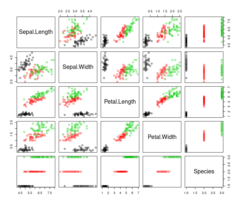
Let's build multiple regression for Iris data set. Prepare data

irisn = iris
irisn[,5] = unclass(iris$Species)

Plot data for multivariate data

plot(irisn, col=irisn$Species)

Build Linear Model for Iris dataset

ml = lm(Species~Sepal.Length+Sepal.Width+Petal.Length+Petal.Width, data=irisn)

Coefficients

coef(ml)

Differences between observed values and fitted values

residuals(ml)[1:10]

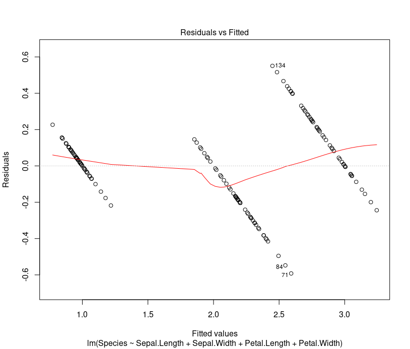
To check for homoscedasticity plot following chart. Residual vs predicted value scatter plot should not look like a funnel.

plot(ml, which=1)

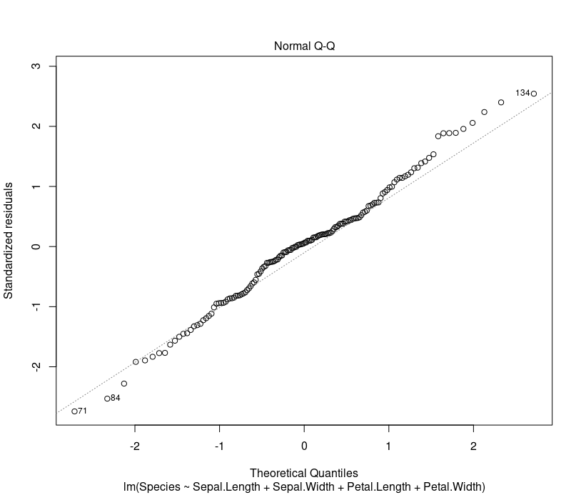
To check if the residuals are approximately normally distributed plot following chart. Q-Q plot should be close to the straight line.

plot(ml, which=2)

To predict Species based on Linear Model using new values for Sepal.Length, Sepal.Width, Petal.Length, Petal.Width

new_data = data.frame(Sepal.Length=5.7, Sepal.Width=3.1, Petal.Length=5.0, Petal.Width=1.7)
predict(ml, new_data)

Calculate the root-mean-square error (RMSE), less is better

RMSE = function(predicted, true) mean((predicted - true)^2)^.5
RMSE(predict(ml, new_data), irisn$Species)

Types of regression

There are different types of regression:

• Linear regression. This is the oldest type and most widely known type of regression. In this the dependent variable is continuous and the independent variable can be discrete or continuous and the regression line is linear. Linear regression is very sensitive to outliers and cross-correlations.
• Logistic regression. This is used when the dependent variable is binary in nature (0 or 1, success or failure, survived or died, yes or no, true or false). It is widely used in clinical trials, fraud detection, and so on. It does not require there to be a linear relationship between dependent and independent variables.
• Polynomial regression. This implies of polynomial equation here the power of the independent variable is more than one. In this case the regression line is not a straight line, but a curved line.
• Ridge regression. This is a more robust version of linear regression and is used when data variables are highly correlated. Using some constraints on regression coefficients, it is made some more natural, closer to real estimates.
• Lasso regression. This is like ridge regression by penalizing the absolute size of regression coefficients. It also automatically performs the variable reduction.
• Ecologic regression. This is used when data is divided in different group or strata, performing regression per group or strata. One should be cautious when using this kind of regression as best regression may get over shadowed by noisy ones.
• Logic regression. This is same as Logistic regression, but it is used in scoring algorithms where all variables are of binary nature.
• Bayesian regression. This uses Bayesian interface of conditional probability. It uses the same approach as ridge regression, which involved penalizing estimator, making it more flexible and stable. It assumes some prior knowledge about regression coefficient and error terms and the error information is loaded with approximated probability distribution.
• Quantile regression. This is used when the area of interest is to study extreme limits, for example pollution level to study interest in death due to pollution. In this conditional quantile function of independent variable is used. It tries to estimate the value with conditional quantiles.
• Jackknife regression. This uses a resampling algorithm to remove the bias and variance.