Density-based clustering in R Science 03.02.2017

Introduction

Clustering is a multivariate analysis used to group similar objects (close in terms of distance) together in the same group (cluster). Unlike supervised learning methods (for example, classification and regression) a clustering analysis does not use any label information, but simply uses the similarity between data features to group them into clusters.

Clustering does not refer to specific algorithms but it’s a process to create groups based on similarity measure. Clustering analysis use unsupervised learning algorithm to create clusters.

Clustering algorithms generally work on simple principle of maximization of intracluster similarities and minimization of intercluster similarities. The measure of similarity determines how the clusters need to be formed.

Similarity is a characterization of the ratio of the number of attributes two objects share in common compared to the total list of attributes between them. Objects which have everything in common are identical, and have a similarity of 1.0. Objects which have nothing in common have a similarity of 0.0.

Clustering can be widely adapted in the analysis of businesses. For example, a marketing department can use clustering to segment customers by personal attributes. As a result of this, different marketing campaigns targeting various types of customers can be designed.

Clustering model is a notion used to signify what kind of clusters we are trying to identify. The four most common models of clustering methods are hierarchical clustering, k-means clustering, model-based clustering, and density-based clustering:

• Hierarchical clustering. It creates a hierarchy of clusters, and presents the hierarchy in a dendrogram. This method does not require the number of clusters to be specified at the beginning. Distance connectivity between observations is the measure.
• k-means clustering. It is also referred to as flat clustering. Unlike hierarchical clustering, it does not create a hierarchy of clusters, and it requires the number of clusters as an input. However, its performance is faster than hierarchical clustering. Distance from mean value of each observation/cluster is the measure.
• Model-based clustering (or Distribution models). Both hierarchical clustering and k-means clustering use a heuristic approach to construct clusters, and do not rely on a formal model. Model-based clustering assumes a data model and applies an EM algorithm to find the most likely model components and the number of clusters. Significance of statistical distribution of variables in the dataset is the measure.
• Density-based clustering. It constructs clusters in regard to the density measurement. Clusters in this method have a higher density than the remainder of the dataset. Density in data space is the measure.

A good clustering algorithm can be evaluated based on two primary objectives:

• High intra-class similarity
• Low inter-class similarity

Density-based clustering uses the idea of density reachability and density connectivity (as an alternative to distance measurement), which makes it very useful in discovering a cluster in nonlinear shapes. This method finds an area with a higher density than the remaining area. One of the most famous methods is Density-Based Spatial Clustering of Applications with Noise (DBSCAN). It uses the concept of density reachability and density connectivity.

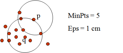
• Density reachability. A point p is said to be density reachable from a point q if point p is within e distance from point q and q has sufficient number of points in its neighbors which are within distance e.
• Density connectivity. A point p and q are said to be density connected if there exist a point r which has sufficient number of points in its neighbors and both the points p and q are within the e distance. This is chaining process. So, if q is neighbor of r, r is neighbor of s, s is neighbor of t which in turn is neighbor of p implies that q is neighbor of p.

The Density-based clustering algorithm DBSCAN is a fundamental data clustering technique for finding arbitrary shape clusters as well as for detecting outliers.

Unlike K-Means, DBSCAN does not require the number of clusters as a parameter. Rather it infers the number of clusters based on the data, and it can discover clusters of arbitrary shape (for comparison, K-Means usually discovers spherical clusters). Partitioning methods (K-means, PAM clustering) and hierarchical clustering are suitable for finding spherical-shaped clusters or convex clusters. In other words, they work well for compact and well separated clusters. Moreover, they are also severely affected by the presence of noise and outliers in the data.

Advantages of Density-based clustering are

1. No assumption on the number of clusters. The number of clusters is often unknown in advance. Furthermore, in an evolving data stream, the number of natural clusters is often changing.
2. Discovery of clusters with arbitrary shape. This is very important for many data stream applications.
3. Ability to handle outliers (resistant to noise).

Disadvantages of Density-based clustering are

1. If there is variation in the density, noise points are not detected
2. Sensitive to parameters i.e. hard to determine the correct set of parameters.
3. The quality of DBSCAN depends on the distance measure.
4. DBSCAN cannot cluster data sets well with large differences in densities.

This algorithm works on a parametric approach. The two parameters involved in this algorithm are:

• e (eps) is the radius of our neighborhoods around a data point p.
• minPts is the minimum number of data points we want in a neighborhood to define a cluster.

One limitation of DBSCAN is that it is sensitive to the choice of e, in particular if clusters have different densities. If e is too small, sparser clusters will be defined as noise. If e is too large, denser clusters may be merged together.

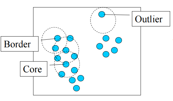
Once these parameters are defined, the algorithm divides the data points into three points:

• Core points. A point p is a core point if at least minPts points are within distance l (l is the maximum radius of the neighborhood from p) of it (including p).
• Border points. A point q is border from p if there is a path p¹, ..., pⁿ with p¹ = p and pⁿ = q, where each pⁱ⁺¹ is directly reachable from pⁱ (all the points on the path must be core points, with the possible exception of q).
• Outliers. All points not reachable from any other point are outliers.

The steps in DBSCAN are simple after defining the previous steps:

1. Pick at random a point which is not assigned to a cluster and calculate its neighborhood. If, in the neighborhood, this point has minPts then make a cluster around that; otherwise, mark it as outlier.
2. Once you find all the core points, start expanding that to include border points.
3. Repeat these steps until all the points are either assigned to a cluster or to an outlier.

Modeling in R

In the following part, we will demonstrate how to use DBSCAN to perform density-based clustering.

# install.packages("dbscan")
library(dbscan)

Determing optimal value of e (eps). First of all, we should define the optimal value of e. The method proposed here consists of computing the he k-nearest neighbor distances in a matrix of points.

The idea is to calculate, the average of the distances of every point to its k nearest neighbors. The value of k will be specified by the user and corresponds to MinPts.

Next, these k-distances are plotted in an ascending order. The aim is to determine the knee” which corresponds to the optimal e parameter.

A knee corresponds to a threshold where a sharp change occurs along the k-distance curve.

The function kNNdistplot() can be used to draw the k-distance plot.

iris_matrix <- as.matrix(iris[, -5])
kNNdistplot(iris_matrix, k=4)
abline(h=0.4, col="red")

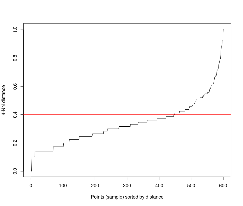
It can be seen that the optimal e value is around a distance of 0.4.

set.seed(1234)
db = dbscan(iris_matrix, 0.4, 4)
db

The result shows DBSCAN has found four clusters and assigned 25 cases as noise/outliers.

Display the hull plot

hullplot(iris_matrix, db$cluster)

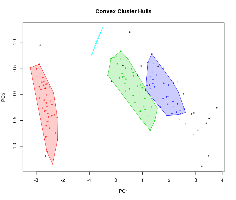
The hull plot shows the separation is good, so we can play around with the parameters to get more generalized or specialized clusters. Black points are outliers.

You can play with e (neighborhood size) and MinPts (minimum of points needed for core cluster).

Compare amount of the data within each cluster

table(iris$Species, db$cluster)

Comparing clustering methods

After fitting data into clusters using different clustering methods, you may wish to measure the accuracy of the clustering. In most cases, you can use either intracluster or intercluster metrics as measurements. The higher the intercluster distance, the better it is, and the lower the intracluster distance, the better it is.

We now introduce how to compare different clustering methods using cluster.stat from the fpc package.

Perform the following steps to compare clustering methods.

First, install and load the fpc package

#install.packages("fpc")
library("fpc")

Next, retrieve the cluster validation statistics of clustering method:

cs = cluster.stats(dist(iris[1:4]), db$cluster)

Most often, we focus on using within.cluster.ss and avg.silwidth to validate the clustering method. The within.cluster.ss measurement stands for the within clusters sum of squares, and avg.silwidth represents the average silhouette width.

• within.cluster.ss measurement shows how closely related objects are in clusters; the smaller the value, the more closely related objects are within the cluster.
• avg.silwidth is a measurement that considers how closely related objects are within the cluster and how clusters are separated from each other. The silhouette value usually ranges from 0 to 1; a value closer to 1 suggests the data is better clustered.

cs[c("within.cluster.ss","avg.silwidth")]

Finally, you can generate the cluster statistics of different clustering method and list them in a table.