Model-based clustering and Gaussian mixture model in R Science 01.02.2017

Introduction

Clustering is a multivariate analysis used to group similar objects (close in terms of distance) together in the same group (cluster). Unlike supervised learning methods (for example, classification and regression) a clustering analysis does not use any label information, but simply uses the similarity between data features to group them into clusters.

Clustering does not refer to specific algorithms but it’s a process to create groups based on similarity measure. Clustering analysis use unsupervised learning algorithm to create clusters.

Clustering algorithms generally work on simple principle of maximization of intracluster similarities and minimization of intercluster similarities. The measure of similarity determines how the clusters need to be formed.

Similarity is a characterization of the ratio of the number of attributes two objects share in common compared to the total list of attributes between them. Objects which have everything in common are identical, and have a similarity of 1.0. Objects which have nothing in common have a similarity of 0.0.

Clustering can be widely adapted in the analysis of businesses. For example, a marketing department can use clustering to segment customers by personal attributes. As a result of this, different marketing campaigns targeting various types of customers can be designed.

Clustering model is a notion used to signify what kind of clusters we are trying to identify. The four most common models of clustering methods are hierarchical clustering, k-means clustering, model-based clustering, and density-based clustering:

• Hierarchical clustering. It creates a hierarchy of clusters, and presents the hierarchy in a dendrogram. This method does not require the number of clusters to be specified at the beginning. Distance connectivity between observations is the measure.
• k-means clustering. It is also referred to as flat clustering. Unlike hierarchical clustering, it does not create a hierarchy of clusters, and it requires the number of clusters as an input. However, its performance is faster than hierarchical clustering. Distance from mean value of each observation/cluster is the measure.
• Model-based clustering (or Distribution models). Both hierarchical clustering and k-means clustering use a heuristic approach to construct clusters, and do not rely on a formal model. Model-based clustering assumes a data model and applies an EM algorithm to find the most likely model components and the number of clusters. Significance of statistical distribution of variables in the dataset is the measure.
• Density-based clustering. It constructs clusters in regard to the density measurement. Clusters in this method have a higher density than the remainder of the dataset. Density in data space is the measure.

A good clustering algorithm can be evaluated based on two primary objectives:

• High intra-class similarity
• Low inter-class similarity

One disadvantage of hierarchical clustering algorithms, k-means algorithms and others is that they are largely heuristic and not based on formal models. Formal inference is not possible.

The key advantage of model-based approach, compared to the standard clustering methods (k-means, hierarchical clustering, etc.), is the suggestion of the number of clusters and an appropriate model.

Instead of taking a heuristic approach to build a cluster, model-based clustering uses a probability-based approach. Model-based clustering assumes that the data is generated by an underlying probability distribution and tries to recover the distribution from the data. One common model-based approach is using finite mixture models, which provide a flexible modeling framework for the analysis of the probability distribution. Finite mixture models are a linearly weighted sum of component probability distribution.

In model-based clustering the data are considered as coming from a distribution that is mixture of two or more components (i.e. clusters). Each component k (i.e. group or cluster) is modeled by the normal or Gaussian distribution which is characterized by the parameters: mean vector, covariance matrix, associated probability (each point has a probability of belonging to each cluster).

Each cluster k is centered at the means, with increased density for points near the mean. Geometric features (shape, volume, orientation) of each cluster are determined by the covariance matrix.

Model-based clustering are iterative method to fit a set of dataset into clusters by optimizing distributions of datasets in clusters. Gaussian distribution is nothing but normal distribution. This method works in three steps:

1. First randomly choose Gaussian parameters and fit it to set of data points.
2. Iteratively optimize the distribution parameters to fit as many points it can.
3. Once it converges to a local minima, you can assign data points closer to that distribution of that cluster.

Although this algorithm create complex models, it does capture correlation and dependence among the attributes. The downside is that these methods usually suffer from an overfitting problem.

Details about Gaussian mixture models

Probabilistic model-based clustering techniques have been widely used and have shown promising results in many applications, ranging from image segmentation, handwriting recognition, document clustering, topic modeling to information retrieval. Model-based clustering approaches attempt to optimize the fit between the observed data and some mathematical model using a probabilistic approach.

The word model is usually used to represent the type of constraints and geometric properties of the covariance matrices.

Such methods are often based on the assumption that the data are generated by a mixture of underlying probability distributions. In practice, each cluster can be represented mathematically by a parametric probability distribution, such as a Gaussian or a Poisson distribution. Thus, the clustering problem is transformed into a parameter estimation problem since the entire data can be modeled by a mixture of k component distributions.

In probabilistic models, the core idea is to model the data from a generative process. First, a specific form of the generative model (e.g., mixture of Gaussians) is assumed, and then the parameters of this model are estimated with the use of the Expectation Maximization (EM) algorithm. The available data set is used to estimate the parameters in such as way that they have a maximum likelihood fit to the generative model. Given this model, we then estimate the generative probabilities (or fit probabilities) of the underlying data points. Data points which fit the distribution well will have high fit probabilities, whereas anomalies will have very low fit probabilities.

In model-based clustering, it is assumed that the data are generated by a mixture of probability distributions in which each component represents a different cluster.

The generative models are typically solved with the use of an EM approach which is the most widely used method for estimating the parameters of a finite mixture probability density. The model-based clustering framework provides a principal way to deal with several problems in this approach, such as the number of component densities (or clusters), initial values of the parameters (the EM algorithm needs initial parameter values to get started), and distributions of the component densities (e.g., Gaussian). EM starts off with a random or heuristic initialization and then iteratively uses two steps to resolve the circularity in computation:

• E-Step. Determine the expected probability of assignment of data points to clusters with the use of current model parameters.
• M-Step. Determine the optimum model parameters of each mixture by using the assignment probabilities as weights.

In the previous article I introduced k-means clustering, which is one of the most widely used approaches for clustering. This non-parametric method for extracting structure has some excellent properties that make it ideal for many situations. In this article, we'll look at a parametric method that uses the Gaussian distribution, known as the Gaussian mixture model (GMM).

You may have heard of the Gaussian distribution, sometimes known as the normal distribution. Qualitatively it can be thought of as a distribution that occurs naturally and very frequently. This has two parameters, which we need to learn in order to fit this equation to our data: the mean and the standard deviation. The mean is a measure of the center of the distribution. The standard deviation is a measure of the distribution of the data around the mean. Armed with the knowledge that, for a normal distribution, 95% of the data is always within two standard deviations from the mean.

Modeling in R

Here, we show example of algorithm on iris dataset.

Mclust package uses Bayesian Information Criterion (BIC) to find the number of clusters (model selection). BIC uses the likelihood and a penalty term to guard against overfitting.

First, install and load the library mclust

#install.packages("mclust")
library(mclust)

You can then perform model-based clustering on the iris dataset using Mclust:

mb = Mclust(iris[,-5])

#or specify number of clusters
mb3 = Mclust(iris[,-5], 3)

# optimal selected model
mb$modelName

# optimal number of cluster
mb$G

# probality for an observation to be in a given cluster
head(mb$z)

# get probabilities, means, variances
summary(mb, parameters = TRUE)

Compare amount of the data within each cluster

table(iris$Species, mb$classification)
# vs
table(iris$Species, mb3$classification)

After the data is fit into the model, we plot the model based on clustering results.

plot(mb, what=c("classification"))

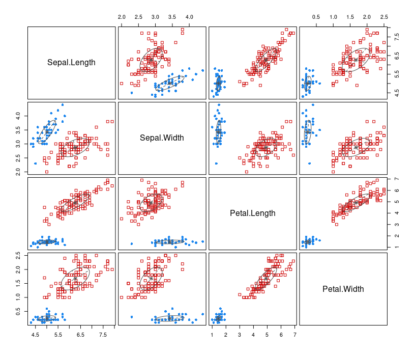
The types of what argument are: "BIC", "classification", "uncertainty", "density". By default, all the above graphs are produced.

Mclust uses an identifier for each possible parametrization of the covariance matrix that has three letters: E for "equal", V for "variable" and I for "coordinate axes". The first identifier refers to volume, the second to shape and the third to orientation. For example:

• EEE means that the G clusters have the same volume, shape and orientation in p−dimensional space.
• VEI means variable volume, same shape and orientation equal to coordinate axes.
• EIV means same volume, spherical shape and variable orientation.

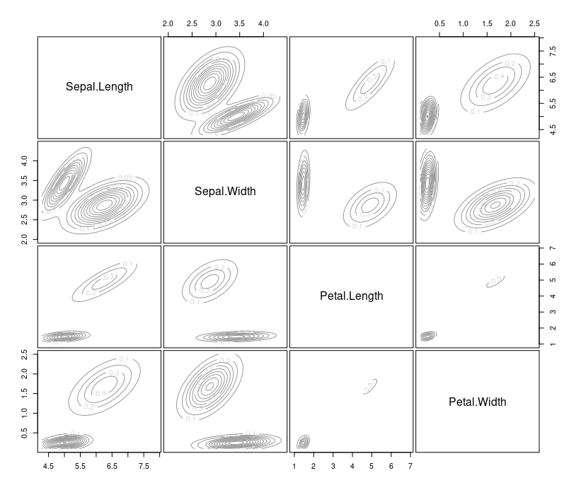
Let's plot estimated density. Contour plot

plot(mb, "density")

You can also use the summary() function to obtain the most likely model and the most possible number of clusters. For this example, the most possible number of clusters is five, with a BIC value equal to -556.1142.

Comparing clustering methods

After fitting data into clusters using different clustering methods, you may wish to measure the accuracy of the clustering. In most cases, you can use either intracluster or intercluster metrics as measurements. The higher the intercluster distance, the better it is, and the lower the intracluster distance, the better it is.

We now introduce how to compare different clustering methods using cluster.stat from the fpc package.

Perform the following steps to compare clustering methods.

First, install and load the fpc package

#install.packages("fpc")
library("fpc")

Next, retrieve the cluster validation statistics of clustering method:

cs = cluster.stats(dist(iris[1:4]), mb$classification)

Most often, we focus on using within.cluster.ss and avg.silwidth to validate the clustering method. The within.cluster.ss measurement stands for the within clusters sum of squares, and avg.silwidth represents the average silhouette width.

• within.cluster.ss measurement shows how closely related objects are in clusters; the smaller the value, the more closely related objects are within the cluster.
• avg.silwidth is a measurement that considers how closely related objects are within the cluster and how clusters are separated from each other. The silhouette value usually ranges from 0 to 1; a value closer to 1 suggests the data is better clustered.

cs[c("within.cluster.ss","avg.silwidth")]

Finally, you can generate the cluster statistics of different clustering method and list them in a table.

The relationship between k-means and GMM

K-means can be expressed as a special case of the Gaussian mixture model. In general, the Gaussian mixture is more expressive because membership of a data item to a cluster is dependent on the shape of that cluster, not just its proximity.

As with k-means, training a Gaussian mixture model with EM can be quite sensitive to initial starting conditions. If we compare and contrast GMM to k-means, we’ll find a few more initial starting conditions in the former than in the latter. In particular, not only must the initial centroids be specified, but the initial covariance matrices and mixture weights must be specified also. Among other strategies, one approach is to run k-means and use the resultant centroids to determine the initial starting conditions for the Gaussian mixture model.

Outcome

A key feature of most clustering algorithms is that every point is assigned to a single cluster. But realistically, many datasets contain a large gray area, and mixture models are a way to capture that.

You can think of Gaussian mixture models as a version of k-means that captures the notion of a gray area and gives confidence levels whenever it assigns a point to a particular cluster.

Each cluster is modeled as a multivariate Gaussian distribution, and the model is specified by giving the following:

1. The number of clusters.
2. The fraction of all data points that are in each cluster.
3. Each cluster’s mean and its d-by-d covariance matrix.

When training a GMM, the computer keeps a running confidence level of how likely each point is to be in each cluster, and it never decides them definitively: the mean and standard deviation for a cluster will be influenced by every point in the training data, but in proportion to how likely they are to be in that cluster. When it comes time to cluster a new point, you get out a confidence level for every cluster in your model.

Mixture models have many of the same blessings and curses of k-means. They are simple to understand and implement. The computational costs are very light and can be done in a distributed way. They provide clear, understandable output that can be easily used to cluster additional points in the future. On the other hand, they both assume more-or-less convex clusters, and they are both liable to fall into local minimums when training.