Classification using k-Nearest Neighbors in R Science 22.01.2017

Introduction

The k-NN algorithm is among the simplest of all machine learning algorithms. It also might surprise many to know that k-NN is one of the top 10 data mining algorithms.

k-Nearest Neighbors algorithm (or k-NN for short) is a non-parametric method used for classification and regression. In both cases, the input points consists of the k closest training examples in the feature space.

Non-parametric means that it does not make any assumptions on the underlying data distribution.

Since the points are in feature space, they have a notion of distance. This need not necessarily be Euclidean distance although it is the one commonly used. Each of the training data consists of a set of vectors and class label associated with each vector. In the simplest case, it will be either + or – (for positive or negative classes). But k-NN, can work equally well with arbitrary number of classes.

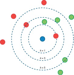
k number decides how many neighbors (where neighbors is defined based on the distance metric) influence the classification. With a given k value we can make boundaries of each class.

For any fixed point x we can calculate how close each observation Xⁱ is to x using the Euclidean distance. This ranks the data by how close they are to x. Imagine drawing a small ball about x and slowly inflating it. As the ball hits the first observation Xⁱ, this is the first nearest neighbor of x. As the ball further inflates and hits a second observation, this observation is the second nearest neighbor.

Efficiency of the k-NN algorithm largely depends on the value of k i.e, choosing the number of nearest neighbors. Choosing the optimal value for k is best done by first inspecting the data. In general, a large k value is more precise as it reduces the overall noise but there is no guarantee. Cross-validation is another way to retrospectively determine a good k value by using an independent dataset to validate the k value. Historically, the optimal k for most datasets has been between 3-10.

k-NN makes predictions using the training dataset directly. Predictions are made for a new instance x by searching through the entire training set for the k most similar instances (the neighbors) and summarizing the output variable for those k instances. For regression this might be the mean output variable, in classification this might be the mode (or most common) class value.

To determine which of the k instances in the training dataset are most similar to a new input a distance measure is used. You can choose the best distance metric based on the properties of your data. Following are the most popular distance measures

• Euclidean distance. This measure is popular for real-valued input variables. The Euclidean distance is always greater than or equal to zero. The measurement would be zero for identical points and high for points that show little similarity. It is a good distance measure to use if the input variables are similar in type (e.g. all measured widths and heights)
• Hamming distance. Calculate the distance between binary vectors.
• Manhattan distance. Calculate the distance between real vectors using the sum of their absolute difference. Also called City Block Distance. It is a good measure to use if the input variables are not similar in type (such as age, gender, height, etc.).
• Minkowski distance. Generalization of Euclidean and Manhattan distance.
• Tanimoto distance is only applicable for a binary variable.
• Jaccard distance measures similarity between finite sample sets, and is defined as the size of the intersection divided by the size of the union of the sample sets.
• Mahalanobis distance
• Cosine distance ranges from +1 to -1 where +1 is the highest correlation. Complete opposite points have correlation -1.

The output of k-NN depends on whether it is used for classification or regression:

• In k-NN classification, the output is a class membership. An object is classified by a majority vote of its neighbors, with the object being assigned to the class most common among its k nearest neighbors (k is a positive integer, typically small).
• In k-NN regression, the output is the property value for the object. This value is the average of the values of its k nearest neighbors.

However, it is more widely used in classification problems in the industry because it's easy of interpretation and low calculation time (for small dataset). The computational complexity of k-NN increases with the size of the training dataset.

k-NN is also a lazy algorithm. What this means is that it does not use the training data points to do any generalization. Lack of generalization means that k-NN keeps all the training data and all the training data is needed during the testing phase. As result:

• more time might be needed as in the worst case, all data points might take point in decision.
• more memory is needed as we need to store all training data.

In k-Nearest Neighbor classification, the training dataset is used to classify each member of a target dataset. The structure of the data is that there is a classification (categorical) variable of interest ("buyer," or "non-buyer," for example), and a number of additional predictor variables (age, income, location, etc).

Before use k-NN we should do some preparations

• Rescale Data. k-NN performs much better if all of the data has the same scale. Normalizing your data to the range [0, 1] is a good idea. It may also be a good idea to standardize your data if it has a Gaussian distribution.
• Address Missing Data. Missing data will mean that the distance between samples can not be calculated. These samples could be excluded or the missing values could be imputed.
• Lower Dimensionality. k-NN is suited for lower dimensional data. You can try it on high dimensional data (hundreds or thousands of input variables) but be aware that it may not perform as well as other techniques. k-NN can benefit from feature selection that reduces the dimensionality of the input feature space.

Following is the algorithm:

1. For each row (case) in the target dataset (the set to be classified), locate the k closest members (the k nearest neighbors) of the training dataset. A Euclidean distance measure is used to calculate how close each member of the training set is to the target row that is being examined.
2. Examine the k nearest neighbors - which classification (category) do most of them belong to? Assign this category to the row being examined.
3. Repeat this procedure for the remaining rows (cases) in the target set.

Modeling in R

Let's see how to use k-NN for classification. In this case, we are given some data points for training and also a new unlabelled data for testing. Our aim is to find the class label for the new point. The algorithm has different behavior based on k.

Before starting with the k-NN implementation using R, I would like to discuss two Data Normalization/Standardization techniques for data consistent. You can easily see this when you go through the results of the summary() function. Look at the minimum and maximum values of all the (numerical) attributes. If you see that one attribute has a wide range of values, you will need to normalize your dataset, because this means that the distance will be dominated by this feature.

• Min-Max Normalization. This process transforms a feature value in such a way that all of its values falls in the range of 0 and 1. This technique is traditionally used with k-Nearest Neighbors classification problems.
• Z-Score Standardization. This process subtracts the mean value of feature x and divides it with the standard deviation of x. The disadvantage with min-max normalization technique is that it tends to bring data towards the mean. If there is a need for outliers to get weighted more than the other values, z-score standardization technique suits better. In order to achieve z-score standardization, one could use R’s built-in scale() function.

To perform a k-nearest neighbour classification in R we will make use of the knn function in the class package and iris data set.

# familiarize with data
str(iris)
table(iris$Species)

The table() function performs a simple two-way cross-tabulation of values. For each unique value of the first variable, it counts the occurrences of different values of the second variable. It works for numeric, factor, and character variables.

A quick look at the Species attribute through tells you that the division of the species of flowers is 50-50-50.

If you want to check the percentual division of the Species attribute, you can ask for a table of proportions:

round(prop.table(table(iris$Species)) * 100, digits = 1)

Also, you can try to get an idea of your data by making some graphs, such as scatter plots. It can be interesting to see how much one variable is affected by another. In other words, you want to see if there is any correlation between two variables.

plot(iris$Sepal.Length, iris$Sepal.Width, col=iris$Species, pch=19)
legend("topright", legend=levels(iris$Species), bty="n", pch=19, col=palette())

You see that there is a high correlation between the Sepal.Length and the Sepal.Width of the Setosa iris flowers, while the correlation is somewhat less high for the Virginica and Versicolor flowers.

To normalize the data use the following function.

normMinMax = function(x) {
  return((x-min(x))/max(x)-min(x))
}

iris_norm <- as.data.frame(lapply(iris[1:4], normMinMax))

Now create training and test data set. Following is random splitting of iris data as 70% train and 30% test data sets.

set.seed(1234)
indexes = sample(2, nrow(iris), replace=TRUE, prob=c(0.7, 0.3))
iris_train = iris[indexes==1, 1:4]
iris_test = iris[indexes==2, 1:4]
iris_train_labels = iris[indexes==1, 5]
iris_test_labels = iris[indexes==2, 5]

Load class package and call knn() function to build the model.

#install.packages("class")
library("class")

iris_mdl = knn(train=iris_train, test=iris_test, cl=iris_train_labels, k=3)

The function knn takes as its arguments a training data set and a testing data set, which we are now going to create.

You can read about Error rate with varying k here.

To evaluate the model, use CrossTable() function in gmodels package.

#install.packages("gmodels")
library("gmodels")
CrossTable(x=iris_test_labels, y=iris_mdl, prop.chisq = FALSE)

Output:

As you can see from the table above the model make one error mistake of predicting as versicolor instead of virginica, whereas rest all the predicted correctly.

Since the data set contains only 150 observations, the model makes only one mistake. There may be more mistakes in huge data. In that case we need to try using different approach like instead of min-max normalization use Z-Score standardization and also vary the values of k to see the impact on accuracy of predicted result.

We would like to determine the misclassification rate for a given value of k. First, build a confusion matrix. When the values of the classification are plotted in a n x n matrix (2x2 in case of binary classification), the matrix is called the confusion matrix. Each column of the matrix represents the number of predictions of each class, while each row represents the instances in the actual class.

CM = table(iris_test_labels, iris_mdl)

Second, build a diagonal mark quality prediction. Applying the diag function to this table then selects the diagonal elements, i.e., the number of points where k-nearest neighbour classification agrees with the true classification, and the sum command simply adds these values up.

accuracy = (sum(diag(CM)))/sum(CM)

The model has a high overall accuracy that is 0.9736842.

Pros and Cons of k-NN algorithm

Pros. The algorithm is highly unbiased in nature and makes no prior assumption of the underlying data. Being simple and effective in nature, it is easy to implement and has gained good popularity.

Cons. Indeed it is simple but k-NN algorithm has drawn a lot of flake for being extremely simple! If we take a deeper look, this doesn’t create a model since there’s no abstraction process involved. Yes, the training process is really fast as the data is stored verbatim (hence lazy learner) but the prediction time is pretty high with useful insights missing at times. Therefore, building this algorithm requires time to be invested in data preparation (especially treating the missing data and categorical features) to obtain a robust model.