Classification using Decision Trees in R Science 09.11.2016

Introduction

Tree based learning algorithms are considered to be one of the best and mostly used supervised learning methods (having a pre-defined target variable).

Unlike other ML algorithms based on statistical techniques, decision tree is a non-parametric model, having no underlying assumptions for the model.

Decision tree are powerful non-linear classifiers, which utilize a tree structure to model the relationships among the features and the potential outcomes. A decision tree classifier uses a structure of branching decisions, which channel examples into a final predicted class value.

This machine-learning approach is used to classify data into classes and to represent the results in a flowchart, such as a tree structure. This model classifies data in a dataset by flowing through a query structure from the root until it reaches the leaf, which represents one class. The root represents the attribute that plays a main role in classification, and the leaf represents the class. The decision tree model follows the steps outlined below in classifying data:

1. It puts all training examples to a root.
2. It divides training examples based on selected attributes.
3. It selects attributes by using some statistical measures.
4. Recursive partitioning continues until no training example remains, or until no attribute remains, or the remaining training examples belong to the same class.

Types of decision tree is based on the type of target variable we have. It can be of two types:

• Classification Trees: where the target variable is categorical and the tree is used to identify the class within which a target variable would likely fall into. For example, the target variable has two value YES or NO.
• Regression Trees: where the target variable is continuous and tree is used to predict it's value.

During the process of analysis, multiple trees may be created. There are several techniques used to create trees. The techniques are called ensemble methods:

• Bagging decision trees. The data is resampled and frequently used to obtain a prediction based on consensus
• Random forest classifier. Used to improve the classification rate.
• Boosted trees. This can be used for regression or classification problems.
• Rotation forest. Uses a technique called Principal Component Analysis (PCA).

From architecture point of view, decision tree is a graph to represent choices and their results in form of a tree. The nodes in the graph represent an event or choice and the edges of the graph represent the decision rules or conditions.

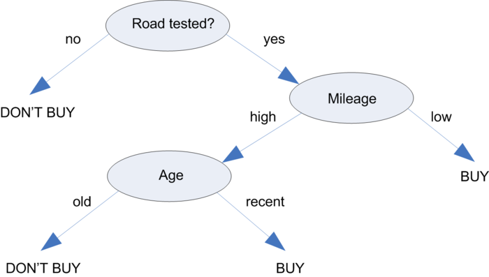
To better understand how this works in practice, let's consider the following tree, which predicts whether a car should be purchased. A car purchase decision begins at the root node, where it is then passed through decision nodes that require choices to be made based on the attributes of the car. These choices split the data across branches that indicate potential outcomes of a decision, depicted here as BUY or DONT'T BUY outcomes, though in some cases there may be more than two possibilities. In the case a final decision can be made, the tree is terminated by leaf nodes (also known as terminal nodes) that denote the action to be taken as the result of the series of decisions. In the case of a predictive model, the leaf nodes provide the expected result given the series of events in the tree.

There are some actions on the tree: splitting is a process of dividing a node into two or more sub-nodes and pruning (opposite process of splitting) is a process when we remove sub-nodes of a decision node.

Another example of decision tree: Is a girl date-worthy?.

Decision trees are built using a heuristic called recursive partitioning. This approach is also commonly known as divide and conquer because it splits the data into subsets, which are then split repeatedly into even smaller subsets, and so on and so forth until the process stops when the algorithm determines the data within the subsets are sufficiently homogenous, or another stopping criterion has been met.

The decision of making strategic splits heavily affects a tree’s accuracy. The decision criteria is different for classification and regression trees.

The algorithm selection (or measuring association between attributes) is also based on type of target variables. Let’s look at the four most commonly used algorithms in decision tree:

• Gini Index is more suitable to continuous attributes and entropy in case of discrete data. Also it works well for minimizing misclassifications.
• Entropy is slightly slower than Gini-index, as it involves logarithms.
• Chi-Square
• Information Gain s a measure that quantifies the change in the entropy before and after the split. It’s an elegantly simple measure to decide the relevance of an attribute.
• Reduction in Variance

There are numerous implementations of decision trees. They differ in the criterion, which decides how to split a variable, the number of splits per step and other details.

• Classification and Regression Trees (CART)
• C4.5
• PART
• Bagging CART
• Random Forest
• Gradient Boosted Machine
• Boosted C5.0

One of the most well-known implementations is the C5.0 algorithm. The C5.0 algorithm has become the industry standard to produce decision trees, because it does well for most types of problems directly out of the box.

Strengths of the C5.0 algorithm

• An all-purpose classifier that does well on most problems
• Highly automatic learning process, which can handle numeric or nominal features, as well as missing data
• Less data cleaning required:
• Excludes unimportant features
• Can be used on both small and large datasets
• Non parametric method (have no assumptions about the space distribution and the classifier structure)
• Results in a model that can be interpreted without a mathematical background (for relatively small trees)
• More efficient than other complex models

Weaknesses of the C5.0 algorithm

• Decision tree models are often biased toward splits on features having a large number of levels
• It is easy to overfit or underfit the model
• Can have trouble modeling some relationships due to reliance on axis-parallel splits
• Small changes in the training data can result in large changes to decision logic
• Large trees can be difficult to interpret and the decisions they make may seem counterintuitive

Modeling in R

There are many packages in R for modeling decision trees: rpart, party, RWeka, ipred, randomForest, gbm, C50.

The R package rpart implements recursive partitioning. The following example uses the iris data set. This dataset contains 3 classes of 150 instances each, where each class refers to the type of the iris plant. We'll try to find a tree, which can tell us if an Iris flower species belongs to one of following classes: setosa, versicolor or virginica. As the response variable is categorial, the resulting tree is called classification tree. The default criterion, which is maximized in each split is the Gini index.

Install and load rpart package

install.packages("rpart")
install.packages("rpart.plot")
library("rpart")
library("rpart.plot")
data("iris")

You can explore iris data set structure by str() command.

str(iris)

Now, we split out entire dataset into two parts - the training set and the testing set. This is a very common practice in machine learning - wherein, we train a machine learning algorithm with the training data, and then test our model using the testing data.

indexes = sample(150, 110)
iris_train = iris[indexes,]
iris_test = iris[-indexes,]

Now, we need to build our decision tree. To do that, we first build a formula which we shall be using to depict the dependencies. For this problem, we're trying to build a model that tries to classify (classification tree) a test data point, into one of the three Species classes - i.e. setosa, virginica or versicolor. The input is a tuple consisting of Sepal.Width, Petal.Width, Sepal.Length and Petal.Length.

target = Species ~ Sepal.Length + Sepal.Width + Petal.Length + Petal.Width

When you set a numerical variable as y value (or target), the tree is a regression tree and you can write the function as below.

target = Sepal.Length ~ ., iris

Build and plot model

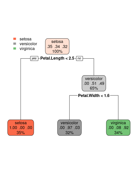
tree = rpart(target, data = iris_train, method = "class")
rpart.plot(tree)

The method argument can be switched according to the type of the response variable. It is class for categorial, anova for numerical, poisson for count data and exp for survival data.

The result is a very short tree: if Petal.Length is smaller than 2.5 we label the flower with setosa. Else we look at the variable Petal.Width. Is Petal.Width smaller than 1.6? If so, we label the flower versicolor, else virginica.

Now that our model is built, we need to cross-check its validity by pitching it against our test data. So we use the predict function to predict the classes of the test data. And then create a matrix showing the comparison between the prediction result and the actual category.

predictions = predict(tree, iris_test)
table(predictions, iris$Species)

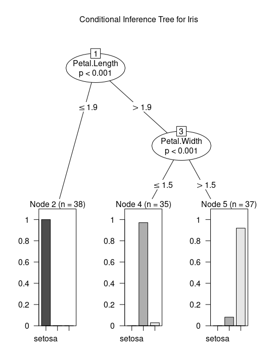
Let's try another package - party. It has ctree() function for fitting conditional trees. Execute ?ctree for the help page. This package has good plotting facilities for conditional trees.

install.packages("party")
library(party)
tree = ctree(Species ~ ., data = iris)
plot(tree, main="Conditional Inference Tree for Iris")
table(predict(tree), iris$Species)

The C5.0 method is a further extension of C4.5 and pinnacle of that line of methods. It is available in the C50 package. The following recipe demonstrates the C5.0 with boosting method applied to the iris dataset.

install.packages("C50")
library(C50)

# build model
tree = C5.0(Species ~ ., data = iris, trials=10)

# make predictions
table(predict(tree, newdata=iris), iris$Species)

Pruning

Size of a decision tree often changes the accuracy of the prediction. In general, bigger tree means higher accuracy, but if the tree is too big, it overfits the data and results in decreased accuracy and robustness. By overfitting, it means the tree may be good at analysing the training data to a high degree of accuracy, but it may fail to correctly predict test data because it is grown with too much features of the training set it is not stable to any minor variations in those features. Robustness means the consistency in the performance of the tree, in this context. Hence, the objective would be to grow a tree to an optimal size that is accurate and robust enough.

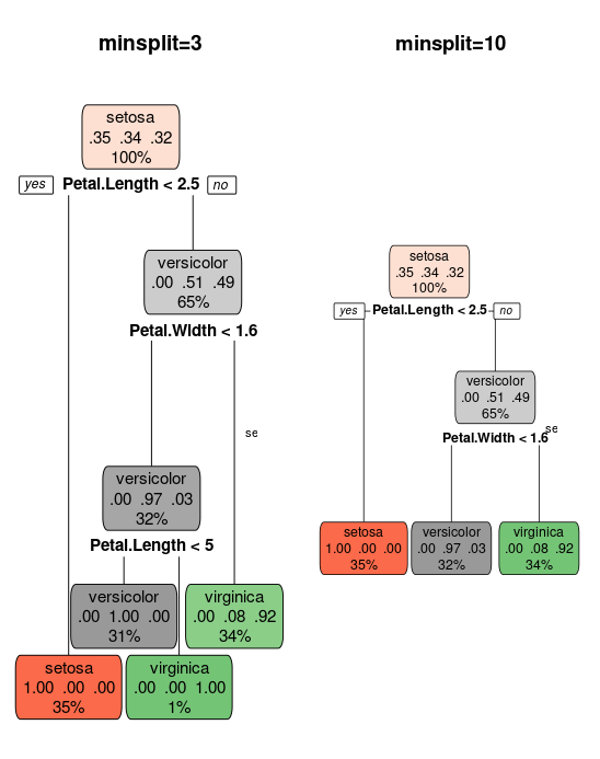
Pruning is a technique used in determining the size of the tree. Often, you would grow a very large tree and starts to trim in down while measuring the change in accuracy and robustness. rpart() offers a parameter minsplit which is used in this pruning process. It refers to minimum number of data points required before a split is made at a node. The below example compares the effect of changing minsplit parameter.

tree_ms3 = rpart(target, iris_train, control = rpart.control(minsplit = 3))
tree_ms10 = rpart(target, iris_train, control = rpart.control(minsplit = 10))

par(mfcol = c(1, 2))
rpart.plot(tree_ms3, main = "minsplit=3")
text(tree_ms3, cex = 0.7)
rpart.plot(tree_ms10, main = "minsplit=10")
text(tree_ms10, cex = 0.7)

Are tree based models better than linear models?

Actually, you can use any algorithm. It is dependent on the type of problem you are solving. Let’s look at some key factors which will help you to decide which algorithm to use:

1. If the relationship between dependent and independent variable is well approximated by a linear model, linear regression will outperform tree based model.
2. If there is a high non-linearity and complex relationship between dependent and independent variables, a tree model will outperform a classical regression method.
3. If you need to build a model which is easy to explain to people, a decision tree model will always do better than a linear model. Decision tree models are even simpler to interpret than linear regression!

Outcome

A decision tree is a tree like chart (tool) showing the hierarchy of decisions and consequences. It is commonly used in decision analysis. Methods of decision tree present their knowledge in the form of logical structures that can be understood with no statistical knowledge.

Interpretation looks like: "If (x1 > 4) and (x2 < 0.5) than (y = 12)". This is much easier to explain to a non-statistician than a linear model. Therefore it is a powerful tool not only for prediction, but also to explain the relation of your response Y and your covariables X in an easy understandable way.

I’d like to point out that a single decision tree usually won’t have much predictive power but an ensemble of varied decision trees such as random forests and boosted models can perform extremely well.

Useful links

• How Decision tree algorithm works