Modeling Self Organising Maps in R Science 29.11.2016

Introduction

The Self-Organizing Maps (SOMs) network is a neural network based method for dimension reduction. SOMs can learn from complex, multidimensional data and transform them into a map of fewer dimensions, such as a two-dimensional plot. The two-dimensional plot provides an easy-to-use graphical user interface to help the decision-maker visualize the similarities between consumer preference patterns.

The SOMs also known as Kohonen Neural Networks is an unsupervised neural network that projects a N-dimensional data set in a reduced dimension space (usually a uni-dimensional (one) or bi-dimensional (two) map). The projection is topological preserving, that is, the proximity among objects in the input space is approximately preserved in the output space. This process, of reducing the dimensionality of vectors, is essentially a data compression technique known as vector quantisation.

The property of topology preserving means that the mapping preserves the relative distance between the points. Points that are near each other in the input space are mapped to nearby map units in the SOMs. The SOMs can thus serve as a cluster analyzing tool of high-dimensional data.

SOMs have been successfully applied as a classification tool to various problem domains, including speech recognition, image data compression, image or character recognition, robot control, and medical diagnosis.

SOMs only operate with numeric variables. Categorical variables must be converted to dummy variables.

The SOMs network typically has two layers of nodes, the input layer (n units, (length of training vectors) and the Kohonen layer (m units, number of categories). The input layer is fully connected to the Kohonen layer. The Kohonen layer, the core of the SOM network, functions similar to biological systems in that it can compress the representation of sparse data and spread out dense data using usually a one- or two-dimensional map. This is done by assigning different subareas of the Kohonen layer to different categories of information and, therefore, the location of the processing element in a network becomes specific to a certain characteristic feature in the set of input data.

Following figure is example of two dimensional SOMs. The network is created from a 2D lattice of 'nodes', each of which is fully connected to the input layer. Figure shows a very small Kohonen network of 4 X 4 nodes connected to the input layer (shown in green) representing a two dimensional vector.

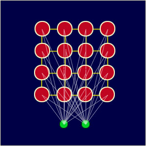
Each node has a specific topological position (an x, y coordinate in the lattice) and contains a vector of weights of the same dimension as the input vectors. That is to say, if the training data consists of vectors, V, of n dimensions:

Then each node will contain a corresponding weight vector W, of n dimensions:

The lines connecting the nodes in figure above are only there to represent adjacency and do not signify a connection as normally indicated when discussing a neural network.

The SOMs is composed of a pre-defined string or grid of N-dimensional units c^(i) that forms a competitive layer, where only one unit responds at the presentation of each input sample x^(m). The activation function is an inverse function of , so that the unit that is closest to x^(m) wins the competition. Here indicates euclidean distance which is the most common way of measuring distance between vectors. The winning unit is then updated according to the relationship

where is the learning rate. However, unlike other competitive methods, each unit is characterised also by its position in the grid.

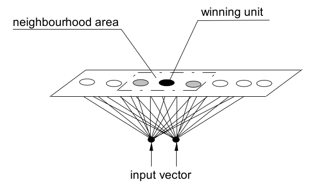
Therefore, the learning algorithm updates not only the weights of the winning unit but also the weights of its neighbour units in inverse proportion of their distance. The neighbourhood size of each unit shrinks progressively during the training process, starting with nearly the whole map and ending with the single unit. In this way, the map auto-organises so that the units that are spatially close correspond to patterns that are similar in the original space. These units form receptive areas, named activity bubbles, that are encircled by units (dead units) that never win the competition for the samples of the training data set. However, the dead units are trained to form a connection zone amongst the activity bubbles and could win for samples not included in the training set.

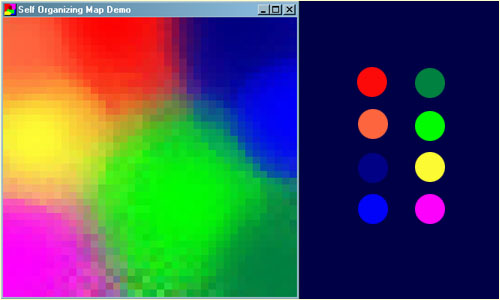
A common example used to help teach the principals behind SOMs is the mapping of colours from their three dimensional components - red, green and blue, into two dimensions. Following figure shows an example of a SOMs trained to recognize the eight different colours shown on the right. The colours have been presented to the network as 3D vectors - one dimension for each of the colour components - and the network has learnt to represent them in the 2D space you can see. Notice that in addition to clustering the colours into distinct regions, regions of similar properties are usually found adjacent to each other. Screenshot of the demo program (left) and the colours it has classified (right).

Training occurs in several steps and over many iterations:

1. Select the size and type of the map. The shape can be hexagonal or square, depending on the shape of the nodes your require. Typically, hexagonal grids are preferred since each node then has 6 immediate neighbours.
2. Initialise all weight vectors randomly.
3. Choose a random datapoint from training data and present it to the SOM.
4. Find the "Best Matching Unit" (BMU) in the map – the most similar node (winning unit).
5. Determine the nodes within the "neighbourhood" of the BMU. The size of the neighbourhood decreases with each iteration.
6. Adjust weights of nodes in the BMU neighbourhood towards the chosen datapoint. The learning rate decreases with each iteration. The magnitude of the adjustment is proportional to the proximity of the node to the BMU.
7. Repeat Steps 3-6 for N iterations / convergence.

SOMs vs k-means

It must be noted that SOM and k-means algorithms are rigorously identical when the radius of the neighborhood function in the SOM equals zero (Bodt, Verleysen et al. 1997).

In a sense, SOMs can be thought of as a spatially constrained form of k-means clustering (Ripley 1996). In that analogy, every unit corresponds to a "cluster", and the number of clusters is defined by the size of the grid, which typically is arranged in a rectangular or hexagonal fashion.

SOMs is less prone to local optima than k-means. During tests it is quite evident that the search space is better explored by SOMs.

If you are interested in clustering/quantization then k-means obviously is not the best choice, because it is sensitive to initialization. SOMs provide a more robust learning. k-means is more sensitive to the noise present in the dataset compared to SOMs.

Modeling in R

The kohonen package is a well-documented package in R that facilitates the creation and visualisation of SOMs.

We'll map the 150-sample iris data set to a map of five-by-five hexagonally oriented units.

# install the kohonen package
install.packages("kohonen")

# load the kohonen package
library("kohonen")

# scale data
iris.sc = scale(iris[, 1:4])

# build grid
iris.grid = somgrid(xdim = 5, ydim=5, topo="hexagonal")

# build model
iris.som = som(iris.sc, grid=iris.grid, rlen=100, alpha=c(0.05,0.01))

The som() function has several parameters. I mention them briefly below. Default values are available for all of them, except the first, the data.

• grid - the rectangular or hexagonal grid of units. The format is the one returned by the function somgrid from the class package.
• rlen - the numer of iterations, i.e. the number of times the data set will be presented to the map. The default is 100.
• alpha - the learning rate, determining the size of the adjustments during training. The decrease is linear, and default values are to start from 0.05 and to stop at 0.01.

The result of the training, the iris.som object, is a list. The most important element is the codes element, which contains the codebook (the data structure that holds the weight vector for each neuron in the grid) vectors as rows. Another element worth inspecting is changes, a vector indicating the size of the adaptions to the codebook vectors during training.

SOMs visualisation are made up of multiple nodes. Typical SOMs visualisations are of heatmaps. A heatmap shows the distribution of a variable across the SOMs. If we imagine our SOMs as a room full of people that we are looking down upon, and we were to get each person in the room to hold up a coloured card that represents their age – the result would be a SOMs heatmap. People of similar ages would, ideally, be aggregated in the same area. The same can be repeated for age, weight, etc. Visualisation of different heatmaps allows one to explore the relationship between the input variables.

The kohonen.plot function is used to visualise the quality of your generated SOMs and to explore the relationships between the variables in your data set. There are a number different plot types available. Understanding the use of each is key to exploring your SOMs and discovering relationships in your data.

Training Progress. As the SOMs training iterations progress, the distance from each node's weights to the samples represented by that node is reduced. Ideally, this distance should reach a minimum plateau. This plot option shows the progress over time. If the curve is continually decreasing, more iterations are required.

plot(iris.som, type="changes")

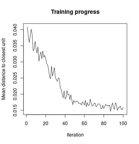
So, the preceding graph explains how the mean distance to the closest unit changes with increase in the iteration level.

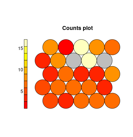
Node Counts. The Kohonen packages allows us to visualise the count of how many samples are mapped to each node on the map. This metric can be used as a measure of map quality – ideally the sample distribution is relatively uniform. Large values in some map areas suggests that a larger map would be beneficial. Empty nodes indicate that your map size is too big for the number of samples. Aim for at least 5-10 samples per node when choosing map size.

plot(iris.som, type="count")

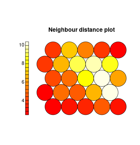
Neighbour Distance. Often referred to as the U-Matrix, this visualisation is of the distance between each node and its neighbours. Typically viewed with a grayscale palette, areas of low neighbour distance indicate groups of nodes that are similar. Areas with large distances indicate the nodes are much more dissimilar – and indicate natural boundaries between node clusters. The U-Matrix can be used to identify clusters within the SOMs map.

plot(iris.som, type="dist.neighbours")

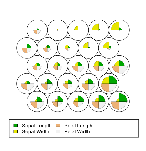
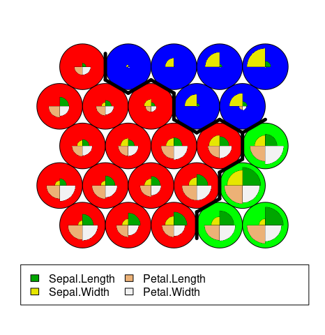
Codes/Weight vectors. The node weight vectors, or codebook, are made up of normalised values of the original variables used to generate the SOM. Each node’s weight vector is representative / similar of the samples mapped to that node. By visualising the weight vectors across the map, we can see patterns in the distribution of samples and variables. The default visualisation of the weight vectors is a fan diagram, where individual fan representations of the magnitude of each variable in the weight vector is shown for each node.

plot(iris.som, type="codes")

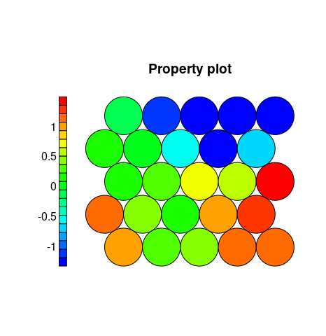
Heatmaps. A SOM heatmap allows the visualisation of the distribution of a single variable across the map. Typically, a SOM investigative process involves the creation of multiple heatmaps, and then the comparison of these heatmaps to identify interesting areas on the map. It is important to remember that the individual sample positions do not move from one visualisation to another, the map is simply coloured by different variables.

The default Kohonen heatmap is created by using the type heatmap, and then providing one of the variables from the set of node weights. In this case we visualise the average Petal.Width level on the SOM.

coolBlueHotRed <- function(n, alpha = 1) {rainbow(n, end=4/6, alpha=alpha)[n:1]}
plot(iris.som, type = "property", property = iris.som$codes[,4], main=names(iris.som$data)[4], palette.name=coolBlueHotRed)

Clustering. The SOMs is comprised of a collection of codebook vectors connected together in a topological arrangement, typically a one dimensional line or a two dimensional grid. The codebook vectors themselves represent prototypes (points) within the domain, whereas the topological structure imposes an ordering between the vectors during the training process. The result is a low dimensional projection or approximation of the problem domain which may be visualized, or from which clusters may be extracted.

## use hierarchical clustering to cluster the codebook vectors
groups = 3
iris.hc = cutree(hclust(dist(iris.som$codes)), groups)

# plot
plot(iris.som, type="codes", bgcol=rainbow(groups)[iris.hc])

#cluster boundaries
add.cluster.boundaries(iris.som, iris.hc)

Outcome

Learning algorithms such as SOMs use an alternative computational model for data processing. Instead of directly manipulating the data, a SOM adapts to the data, or, using the standard terminology, learns from the data. This computational model offers a certain flexibility, which can be used to develop fast and robust data processing algorithms.

The SOMs was designed for unsupervised learning problems such as feature extraction, visualization and clustering. Some extensions of the approach can label the prepared codebook vectors which can be used for classification.

So, SOMs are an unsupervised data visualisation technique that can be used to visualise high-dimensional data sets in lower (typically 2) dimensional representations.

Also, the SOMs has the capability to generalize. Generalization capability means that the network can recognize or characterize inputs it has never encountered before. A new input is assimilated with the map unit it is mapped to.

Advantages os SOMs include:

• Intuitive method to develop segmentation.
• Relatively simple algorithm, easy to explain results to non-data scientists.
• New data points can be mapped to trained model for predictive purposes.

Disadvantages include:

• Lack of parallelisation capabilities for very large data sets.
• Difficult to represent very many variables in two dimensional plane.
• Requires clean, numeric data.