Getting started with Deep learning in R Science 15.06.2016

Introduction

Deep learning is an area of machine learning that emerged from the intersection of neural networks, artificial intelligence, graphical modeling, optimization, pattern recognition and signal processing.

Deep learning is about supervised or unsupervised learning from data using multiple layered machine learning models. The layers in these models consist of multiple stages of nonlinear data transformations, where features of the data are represented at successively higher, more abstract layers.

Input data is passed to the model and filtered through multiple non-linear layers. The final layer consists of a classifier which determines which class the object of interest belongs to.

There are two basic types of learning used in data science

• Supervised learning. Your training data contain the known outcomes. The model is trained relative to these outcomes.
• Unsupervised learning. Your training data does not contain any known outcomes. In this case the algorithm self-discovers relationships in your data.

The goal in learning from data is to predict a response variable or classify a response variable using a group of given attributes. This is somewhat similar to what you might do with linear regression, where the dependent variable (response) is predicted by a linear model using a group of independent variables (aka attributes or features). However, traditional linear regression models are not considered deep because they don't apply multiple layers of non-linear transformation to the data.

Other popular learning from data techniques such as decision trees, random forests and support vector machines, single hidden layer neural networks are not deep.

The power of deep learning models comes from their ability to classify or predict nonlinear data using a modest number of parallel nonlinear steps. A deep learning model learns the input data features hierarchy all the way from raw data input to the actual classification of the data. Each layer extracts features from the output of the previous layer.

Deep multi-layer neural networks contain many levels of nonlinearities which allow them to compactly represent highly non-linear and/or highly-varying functions. They are good at identifying complex patterns in data and have been set work to improve things like computer vision and natural language processing, and to solve unstructured data challenges.

Deep learning is a vast subject and is an important concept for building AI. It is used in various applications, such as:

• Image recognition
• Computer vision
• Handwriting detection
• Text classification
• Multiclass classification
• Regression problems, and more

Microsoft, Google, IBM, Yahoo, Twitter, Baidu, Paypal and Facebook are all exploiting deep learning to understand user’s preferences so that they can recommend targeted ser-vices and products.

About artificial neural network

An Artificial Neural Network (ANN) models highly complex relationships between inputs/features and response variable(s), especially if the relationships are highly nonlinear. No underlying assumptions are required to create and evaluate the model and it can be used with qualitative and quantitative responses.

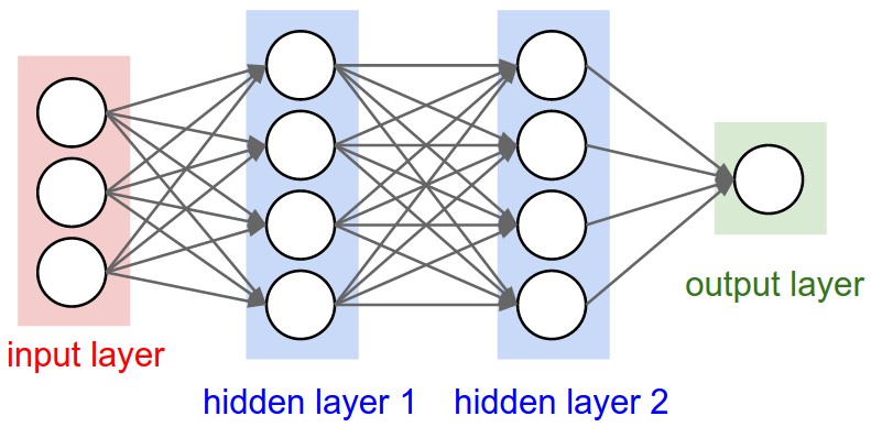
At the heart of an artificial neural network is a mathematical node, unit or neuron. It is the basic processing element. The input layer neurons receive incoming information which they process via a mathematical function and then distribute to the hidden layer neurons. This information is processed by the hidden layer neurons and passed onto the output layer neurons. The key here is that information is processed via an activation function. The activation function emulates brain neurons in that they are fired or not depending on the strength of the input signal.

The result of this processing is then weighted and distributed to the neurons in the next layer. In essence, neurons activate each other via weighted sums. This ensures the strength of the connection between two neurons is sized according to the weight of the processed information.

The model of a single artificial neuron can be understood in the following figure. A directed network diagram defines a relationship between the input signals (x variables), and the output signal (y variable). Each input signal is weighted (w values) according to its importance - ignore. The input signals are summed by the cell body and the signal is passed on according to an activation function denoted by f.

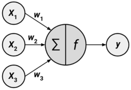
A typical artificial neuron with n inputs can be represented by the formula that follows. The w weights allow each of the n inputs (denoted by x_i) to contribute a greater or lesser amount to the sum of input signals. The net total is used by the activation function f(x), and the resulting signal, y(x), is the output.

Neural networks use neurons defined this way as building blocks to construct complex models of data. Although there are numerous variants of neural networks, each can be defined in terms of the following characteristics:

• An activation function, which transforms a neuron's combined input signals into a single output signal to be broadcasted further in the network.
• A network topology (or architecture), which describes the number of neurons in the model as well as the number of layers and manner in which they are connected.
• The training algorithm that specifies how connection weights are set in order to inhibit or excite neurons in proportion to the input signal.

Each neuron contains an activation function and a threshold value. Activation functions for the hidden layer nodes are needed to introduce non linearity into the network.

There are a wide number of activation functions: linear function, hyperbolic tangent function, sigmoid function, softmax function, rectified linear unit (ReLU), etc.

The threshold value is the minimum value that a input must have to activate the neuron. The task of the neuron therefore is to perform a weighted sum of input signals and apply an activation function before passing the output to the next layer.

To learn from data a neural network uses a specific learning algorithm. There are many learning algorithms, but in general, they all train the network by iteratively modifying the connection weights until the error between the output produced by the network and the desired output falls below a pre-specified threshold.

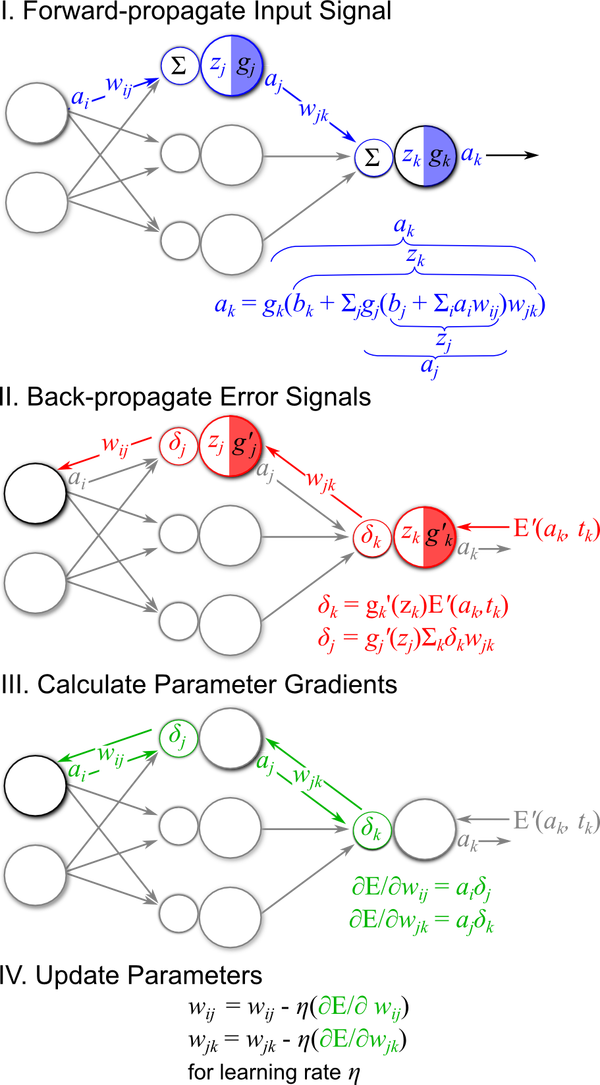
The backpropagation algorithm was the first popular leaning algorithm and is still widely used. It uses gradient descent as the core learning mechanism. Starting from random weights the backpropagation algorithm calculates the network weights making small changes and gradually making adjustments determined by the error between the result produced by the network and the desired outcome.

The algorithm applies error propagation from outputs to inputs and gradually fine tunes the network weights to minimize the sum of error using the gradient descent technique. Learning therefore consists of the following steps.

Multilayer feedforward networks that use the backpropagation algorithm are now common in the field of data mining. Such models offer the following strengths and weaknesses:

A feedforward neural network (FNN) is one of the earliest and simplest dynamic neural networks which can continue learning after the training phase. They can make adjustments to their structure independently of external modification.

Strengths of feedforward networks that use the backpropagation algorithm

• Can be adapted to classification or numeric prediction problems.
• Capable of modeling more complex patterns than nearly any algorithm.
• Makes few assumptions about the data's underlying relationships.

Weaknesses of feedforward networks that use the backpropagation algorithm

• Extremely computationally intensive and slow to train, particularly if the network topology is complex.
• Very prone to overfitting training data.
• Results in a complex black box model that is difficult, if not impossible, to interpret.

Taxonomy of neural networks

The basic foundation for ANNs is the same, but various neural network models have been designed during its evolution. The following are a few of the ANN models:

• Adaptive Linear Element (ADALINE), is a simple perceptron which can solve only linear problems. Each neuron takes the weighted linear sum of the inputs and passes it to a bi-polar function, which either produces a +1 or -1 depending on the sum. The function checks the sum of the inputs passed and if the net is >= 0, it is +1, else it is -1.
• Multiple ADALINEs (MADALINE), is a multilayer network of ADALINE units.
• Perceptrons are single layer neural networks (single neuron or unit), where the input is multidimensional (vector) and the output is a function on the weight sum of the inputs.
• Radial basis function network is an ANN where a radial basis function is used as an activation function. The network output is a linear combination of radial basis functions of the inputs and some neuron parameters.
• Feed-forward is the simplest form of neural networks. The data is processed across layers without any loops are cycles. There are the following feed forward networks: Autoencoder, Probabilistic, Time delay, Covolutional.
• Recurrent Neural Networks (RNNs), unlike feed-forward networks, propagate data forward and also backwards from later processing stages to earlier stages. The following are the types of RNNs: Hopfield networks, Boltzmann machine, Self Organizing Maps (SOMs), Bidirectional Associative Memory (BAM), Long Short Term Memory (LSTM).

Kinds of Deep Neural Networks (DNN)

There are many variations of DNNs, as illustrated by the different terms shown next:

• Deep Belief Network (DBN). It is typically a feed-forward network in which data flows from one layer to another without looping back. There is at least one hidden layer and there can be multiple hidden layers, increasing the complexity.
• Restricted Boltzmann Machine (RBM). It has a single hidden layer and there is no connection between nodes in a group. It is a simple MLP model of neural networks.
• Recurrent Neural Networks (RNN) and Long Short Term Memory (LSTM). These networks have data flowing in any direction within groups and across groups.

Example

So, deep learning neural networks are useful in areas where classification and/ or prediction is required.

There are several packages in R for neural networks: nnet, neuralnet, RSNNS.

Numeric prediction problem.

First we need to load the required packages. For this example, we will use the neuralnet package

# install.packages('neuralnet')
library('neuralnet')

We will build a DNN to approximate . First we create the attribute variable x (or feature), and the response variable y (or target).

set.seed(2016)

# generates 50 observations without replacement over the range -2 to +2
attribute = as.data.frame(sample(seq(-2, 2, length=50), 50, replace=FALSE), ncol=1)

response = attribute^2

Next we combine the attribute and response objects into a dataframe called data

data = cbind(attribute, response)
colnames(data) = c('attribute', 'response')

Let’s take a peek at the first ten observations in data

head(data, 10)

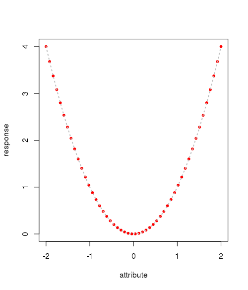
A visual plot of the simulated data is shown below

plot(data, pch=20, col=2)

# draw line
x = data$attribute[order(data$attribute)]
y = data$response[order(data$attribute)]
lines(x, y, col=8, lty=3, lwd=2)

We will fit a DNN with two hidden layers each containing three neurons

fit = neuralnet(response~attribute, data=data, hidden=c(3, 3), threshold =0.01, act.fct="logistic")

The fitted model is shown below

plot(fit)

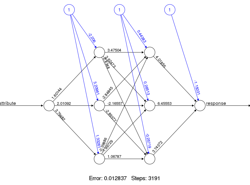
Notice that the image shows the weights of the connections and the intercept or bias weights. Overall, it took 3191 steps for the model to converge with an error of 0.012837.

A bias unit is a neuron that has a constant output. It is always one and is sometimes referred to as a fake node. This neuron is similar to an offset and is essential for most networks to function properly. You could compare the bias neuron to the y-intercept of a linear function in slope-intercept form.

Let’s see how good the model really is at approximating a function using a test sample. We generate 10 observations from the range -2 to +2 and store the result in the testdata

testdata = as.matrix(sample(seq(-2, 2, length =10), 10, replace=FALSE), ncol =1)

Prediction in the neuralnet package is achieved using the compute function

pred = compute(fit, testdata)

The predicted values are accessed from pred using $net.result.

Because this is a numeric prediction problem rather than a classification problem, we cannot use a confusion matrix to examine model accuracy. Instead, we must measure the correlation between our predicted concrete strength and the true value. This provides insight into the strength of the linear association between the two variables.

Recall that the cor() function is used to obtain a correlation between two numeric vectors:

cor(pred$net.result, testdata^2)

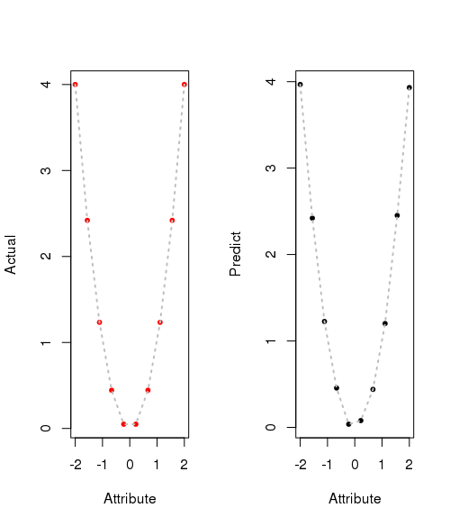
Correlations close to 1 indicate strong linear relationships between two variables. Therefore, the correlation here of about 0.999 indicates a fairly strong relationship. This implies that our model is doing a fairly good job.

Let's plot actual result and predicted result.

result = cbind(testdata, pred$net.result, testdata^2)
colnames(result) = c('Attribute', 'Prediction', 'Actual')
round(result, 4)

# prepare data for plot 
x = result[,"Attribute"][order(result[,"Attribute"])]
y_act = result[,"Actual"][order(result[,"Attribute"])]
y_pred = result[,"Prediction"][order(result[,"Attribute"])]

par(mfrow=c(1,2))

# plot actual data
plot(x, y_act, pch=20, col=2, xlab='Attribute', ylab="Actual")
lines(x, y_act, col=8, lty=3, lwd=2)

# plot predict data
plot(x, y_pred, pch=20, col=1, xlab='Attribute', ylab="Predict")
lines(x, y_pred, col=8, lty=3, lwd=2)

Classification problem.

Artificial neural networks are commonly used for classification in data science. They group feature vectors into classes, allowing you to input new data and find out which label fits best. This can be used to label anything, like customer types or music genres. In engineering, classifiers are often used to diagnose the health of equipment, identifying it as normal, suspect, or faulty.

I'll use the Iris data set to perform this classification. The Iris data set is a classic data set that is often used to demonstrate machine learning. This data set provides four measurements for three different iris species.

Once neuralnet library has been instaled and data set has been downloaded we are ready to go.

install.packages('neuralnet')

The first step is to import the library:

library('neuralnet')

We can now use our neural network. But we need some parameters first, like the number of hidden layers and nodes in each one, the training set, and class labels, we can do it as follows.

# 2 hidden layers with 3 and 4 nodes respectively
hidd = c(3, 4)

It is often useful to break the data into training and validation sets. This allows you to validate the ANN on data that it was never trained with. The Iris data set has 150 elements in it. For our training set we will sample 70 elements from this 150 element set. This is done with the following commands.

indexesTrain = sample(1:150, 70)
indexesValidate = setdiff(1:150, indexesTrain)

train = iris[indexesTrain,]

# classes labeling
train$setosa = c(train$Species == "setosa")
train$versicolor = c(train$Species == "versicolor")
train$virginica = c(train$Species == "virginica")

And now we can train our NN with the next line:

fit = neuralnet(setosa + versicolor + virginica ~ Sepal.Length + Sepal.Width + Petal.Length + Petal.Width, train, hidden=hidd, lifesign="full")

After it is trained, we can validate it.

predict = compute(fit, iris[1:4])

Note the compute function, which receives the NN and the set to validate. In this case, our validation set is the whole data set, from column 1 to 4.

Now to see the results, we can just check the predict variable, in predict$net.result, and those are the predicted results for each sample in the data set.

maxidx = function(arr) {
    return(which(arr == max(arr)))
}
idx = apply(predict$net.result, c(1), maxidx)
prediction = c('setosa', 'versicolor', 'virginica')[idx]
table(prediction, iris$Species)

Also, we can use nnet package to classify Iris data set. But this package use single-hidden-layer neural network. For following example our ANN will have four input units, ten hidden units and 3 output units.

install.packages('nnet')
library(nnet)

The neural network requires that the species be normalized using one-of-n normalization. We will normalize between 0 and 1. This can be done with the following command.

targets = class.ind(iris$Species)

We can now train a neural network for the training data.

fit2 = nnet(train[, -5], targets[indexesTrain,], size=10, softmax=TRUE)

Now we can test the output from the neural network.

predict(irisANN, irisdata[irisValData,-5], type="class")

How many neurons to include

One idea is to use more neurons per layer to detect finer structure in your data. However, the more hidden neurons used the more likely is the risk of over fitting. Over-fitting occurs because with more neurons there is an increased likelihood that the DNN will learn both patterns and noise, rather than the underlying statistical structure of the data. The result is a DNN which performs extremely well in sample but poorly out of sample.

Here is the key point to keep in mind as you build your DNN models. For the best generalization ability, a DNN should have as few neurons as possible to solve the problem at hand with a tolerable error. The larger the number of training patterns, the larger the number of neurons that can be used whilst still preserving the generalization ability of a DNN.

The best number of hidden units depends in a complex way on:

• the numbers of input and output units
• the number of training cases
• the amount of noise in the targets
• the complexity of the function or classification to be learned
• the architecture
• the type of hidden unit activation function
• the training algorithm
• regularization

Other neural networks in short

• Elman neural networks are useful in applications where we are interested in predicting the next output in given sequence. Their dynamic nature can capture time-dependent patterns, which are important for many practical applications. This type of flexibility is important in the analysis of time series data.
• Jordan neural networks appear capably of modeling timeseries data and are useful for classification problems.

Recurrent Neural Networks (RNN). RNN differ from feed-forward networks in that their input includes the input from the previous iteration or step. They still process the current input but use a feedback loop to take into consideration the inputs to the prior step, also called the recent past, for context. This step effectively gives the network memory. One popular type of recurrent network involves Long Short-Term Memory (LSTM). This type of memory improves the processing power of the network.

RNNs are designed to process sequential data and are especially useful for analysis and prediction with text data. Given a sequence of words, an RNN can predict the probability of each word being the next in the sequence. This also allows for text generation by the network. RNNs are versatile and also process image data well, especially image labeling applications. The flexibility in design and purpose and ease in training make RNNs popular choices for many data science applications.

Outcome

ANNs are a powerful technique used to solve many real-world problems such as classification, regression, and feature selection. It consists of layers associated with weights. ANNs have the ability to learn from new experiences in the form of new input data in order to improve the performance of classification- or regression-based tasks and to adapt themselves to changes in the input environment.

ANNs are best applied to problems where the input data and output data are well-defined or at least fairly simple, yet the process that relates the input to output is extremely complex. As a black box method, they work well for these types of black box problems.

The following are some of the advantages of neural networks:

• Neural networks are flexible and can be used for both regression and classification problems. Any data which can be made numeric can be used in the model, as neural network is a mathematical model with approximation functions.
• Neural networks are good to model with nonlinear data with large number of inputs; for example, images. It is reliable in an approach of tasks involving many features. It works by splitting the problem of classification into a layered network of simpler elements.
• Once trained, the predictions are pretty fast.
• Neural networks can be trained with any number of inputs and layers.
• Neural networks work best with more data points.

Let us take a look at some of the cons of neural networks:

• Neural networks are black boxes, meaning we cannot know how much each independent variable is influencing the dependent variables.
• It is computationally very expensive and time consuming to train with traditional CPUs.
• Neural networks depend a lot on training data. This leads to the problem of over-fitting and generalization. The mode relies more on the training data and may be tuned to the data.

Useful book

• Deep Learning Made Easy with R: A Gentle Introduction For Data Science