How-to simulate Support Vector Machine (SVM) in R

How-to simulate Support Vector Machine (SVM) in R Science 22.04.2014

Introduction

Support Vector Machine (SVM) is a supervised machine learning algorithm which can be used for classification or regression problems (numeric prediction).

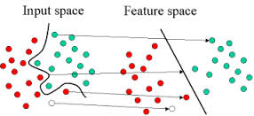
Given a set of training examples, where each data point falls into one of two categories, an SVM training algorithm builds a model that assigns new data points into one category or the other. This model is a representation of the examples as a points in space, mapped so that the examples of the separate categories are divided by a margin that is as wide as possible, as shown in the following image. New examples are then mapped into that same space and predicted to belong to a category based on which side of the gap they fall on.

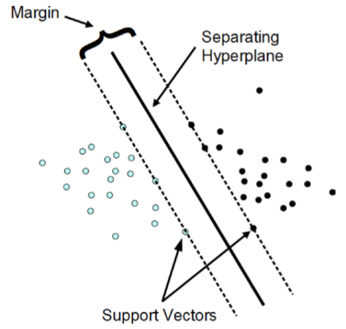
The approach creates a hyperplane to categorize the training data. A hyperplane can be envisioned as a geometric plane that separates two regions. In a two-dimensional space, it will be a line. In a three-dimensional space, it will be a two-dimensional plane. For higher dimensions, it is harder to conceptualize, but they do exist.

SVM looks for the optimal hyperplane separating the two classes by maximizing the margin between the closest points of the two classes. In two-dimensional space, as shown in figure below, the points lying on the margins are called support vectors and line passing through the midpoint of margins is the optimal hyperplane. In two dimensions, a hyperplane is a line and in a p-dimensional space, a hyperplane is a flat affine subspace of hyperplane dimension p - 1.

A SVM can be imagined as a surface that creates a boundary between points of data plotted in multidimensional that represent examples and their feature values. The goal of a SVM is to create a flat boundary called a hyperplane, which divides the space to create fairly homogeneous partitions on either side. In this way, the SVM learning combines aspects of both the instance-based nearest neighbor learning and the linear regression modeling. The combination is extremely powerful, allowing SVMs to model highly complex relationships.

Support vectors are data points that lie near the hyperplane. SVM uses a technique called the kernel trick to transform your data and then based on these transformations it finds an optimal boundary between the possible outputs. Simply put, it does some extremely complex data transformations, then figures out how to seperate your data based on the labels or outputs you've defined.

A few of the most commonly used kernel functions are listed as follows.

The linear kernel does not transform the data at all.
The polynomial kernel of degree d adds a simple nonlinear transformation of the data.
The sigmoid kernel results in a SVM model somewhat analogous to a neural network using a sigmoid activation function.
The Gaussian RBF kernel is similar to a RBF neural network. The RBF kernel performs well on many types of data and is thought to be a reasonable starting point for many learning tasks.

Math background you can find here.

Advantages and Disadvantages of SVM

An important benefit of the support vector machine approach is that the complexity of the resulting classifier is characterised by the number of support vectors rather than the dimensionality of the transformed space. As a result, support vector machines tend to be less prone to problems of over-fitting than some other methods.

There are four main advantages: Firstly it has a regularisation parameter, which makes the user think about avoiding over-fitting. Secondly it uses the kernel trick, so you can build in expert knowledge about the problem via engineering the kernel. Thirdly an SVM is defined by a convex optimisation problem (no local minima) for which there are efficient methods (e.g. SMO). Lastly, it is an approximation to a bound on the test error rate, and there is a substantial body of theory behind it which suggests it should be a good idea. Source.

The disadvantages are that the theory only really covers the determination of the parameters for a given value of the regularisation and kernel parameters and choice of kernel. In a way the SVM moves the problem of over-fitting from optimising the parameters to model selection. Sadly kernel models can be quite sensitive to over-fitting the model selection criterion, see

Compare SVM with NN (neural network) (source)

Similarity

SVM + sigmoid kernel ~ two-layer feedforward NN
SVM + Gaussian kernel ~ RBF network
For most problems, SVM and NN have similar performance

Advantages

Based on sound mathematics theory
Learning result is more robust
Over-fitting is not common
Not trapped in local minima (because of QP)
Fewer parameters to consider (kernel, error cost C)
Works well with fewer training samples (number of support vectors do not matter much)
Can be used for classification or numeric prediction problems
May be easier to use than neural networks, particularly due to the existence of several well-supported SVM algorithms

Disadvantages

Problem need to be formulated as 2-class classification
Learning takes long time (QP optimization)
Difficult to understand the learned function (weights)
Finding the best model requires testing of various combinations of kernels and model parameters
Can be slow to train, particularly if the input dataset has a large number of features or examples
Results in a complex black box model that is difficult, if not impossible, to interpret

Multi-Class SVM

Most popular usage of SVM is as a binary classifier. However the idea of SVM can be extended to multi-class classification problem as well. Multi-class SVM can be used as a multi-class classifier by creating multiple binary classifiers. This method works similarly to the idea of multinomial logistic regression, where we build a logistic model for each pair of class with base function.

We can create a set of binary SVMs to do multi-class classification. The steps in implementing that will be as follows:

Create binary classifiers:
- Between one class and the rest of the classes.
- Between every pair of classes (all possible pairs).
For any new cases, the SVM classifier adopts a winner-takes-all strategy, in which the class with highest output is assigned.

To implement this methodology, it is important that the output functions are calibrated to generate comparable scores, otherwise the classification will become biased.

There are other methods also for multi-class SVMs. One such is proposed by Crammer and Singer. They proposed a multi-class SVM method which casts the multiclass classification problem into a single optimization problem, rather than decomposing it into multiple binary classification problems.

We will show quick example with iris data. The iris$Species is divided into three classes: setosa, versicolor, and virginica. The multi-class SVM has to classify iris into these categories.

Here is the R implementation of the SVM multi-class classifier:

#install.packages("e1071")
library("e1071")

iris_mdl = svm(Species ~ ., data=iris, header=T)
iris_predict = predict(iris_mdl, newdata=iris)
table(iris$Species, iris_predict)
classification_rate = sum(diag(table(iris$Species, iris_predict))) / nrow(iris)

Multi-class SVM gives us 97% good classification_rate on iris data. The prediction is good across all the classes.

A number of applications of SVM emerged over the years, and a few noteworthy ones are hypertext categorization, image classification, character recognition, and many more applications in biological sciences as well.

Modeling SVM in R

Good explanation of modeling SVM in R you can find in

Useful links

How-to simulate Support Vector Machine (SVM) in R Science 22.04.2014

Quote

Categories

Archive ↓