An overview of a Market Basket Analysis (Association Mining) in R Science 20.07.2018

Market basket analysis is a data mining technique that has the purpose of finding the optimal combination of products or services and allows marketers to exploit this knowledge to provide recommendations, optimize product placement, or develop marketing programs that take advantage of cross-selling. In short, the idea is to identify which items go well together, and profit from it.

You can think of the results of the analysis as an if ... then statement. If a customer buys an airplane ticket, then there is a 46 percent probability that they will buy a hotel room, and if they go on to buy a hotel room, then there is a 33 percent probability that they will rent a car.

There are many ways to see the similarities between items. These are techniques that fall under the general umbrella of association. The outcome of this type of technique, in simple terms, is a set of rules that can be understood as "if this, then that".

However, it is not just for sales and marketing. It is also being used in fraud detection and healthcare; for example, if a patient undergoes treatment A, then there is a 26 percent probability that they might exhibit symptom X. The following measures are used to evaluate the strength of association. Suppose, you are interested in the association between two events A and B:

• Itemset: This is a collection of one or more items in the dataset.
• Support: This is the proportion of the transactions in the data that contain an itemset of interest. Support = Number of Rows having both A AND B / Total Number of Rows.
• Confidence: This is the conditional probability that if a person purchases or does x, they will purchase or do y; the act of doing x is referred to as the antecedent or Left-Hand Side (LHS), and y is the consequence or Right-Hand Side (RHS). Confidence = Number of Rows having both A AND B / Number of Rows with A. Expected Confidence = Number of rows with B / Total Number of Rows.
• Lift: This is the ratio of the support of x occurring together with y divided by the probability that x and y occur if they are independent. It is the confidence divided by the probability of x times the probability of y; for example, say that we have the probability of x and y occurring together as 10 percent and the probability of x is 20 percent and y is 30 percent, then the lift would be 10 percent (20 percent times 30 percent) or 16.67 percent. Lift = Confidence / Expected Confidence.
• Rule: A rule is a notation that represents which item/s is frequently bought with what item/s. It has an LHS and an RHS part and can be represented as follows: itemset A => itemset B. This means, the item/s on the right were frequently purchased along with items on the left.

The package in R that you can use to perform a market basket analysis is arules: Mining Association Rules and Frequent Itemsets. The package offers two different methods of finding rules. The algorithms that the package supports are apriori and ECLAT. There are other algorithms to conduct a market basket analysis, but apriori is used most frequently, and so, that will be our focus.

With apriori, the principle is that, if an itemset is frequent, then all of its subsets must also be frequent. A minimum frequency (support) is determined by the analyst prior to executing the algorithm, and once established, the algorithm will run as follows:

• Let k=1 (the number of items)
• Generate itemsets of a length that are equal to or greater than the specified support
• Iterate k + (1...n), pruning those that are infrequent (less than the support)
• Stop the iteration when no new frequent itemsets are identified

Once you have an ordered summary of the most frequent itemsets, you can continue the analysis process by examining the confidence and lift in order to identify the associations of interest.

For our example, we will focus on identifying the association rules for a grocery store. The dataset will be from the arules package and is called Groceries. This dataset consists of actual transactions over a 30-day period from a real-world grocery store and consists of 9,835 different purchases. All the items purchased are put into one of 169 categories, for example, bread, wine, meat, and so on.

For this analysis, we will only need to load two packages, as well as the Groceries dataset:

#install.packages("arules")
#install.packages("arulesViz")
library(arules)
library(arulesViz)
data(Groceries)
head(Groceries)

This dataset is structured as a sparse matrix object, known as the transaction class.

So, once the structure is that of the class transaction, our standard exploration techniques will not work, but the arules package offers us other techniques to explore the data.

The best way to explore this data is with an item frequency plot using the itemFrequencyPlot() function in the arules package. You will need to specify the transaction dataset, the number of items with the highest frequency to plot, and whether or not you want the relative or absolute frequency of the items. Let's first look at the absolute frequency and the top 10 items only:

itemFrequencyPlot(Groceries, topN = 10, type = "absolute")

The output of the preceding command is as follows:

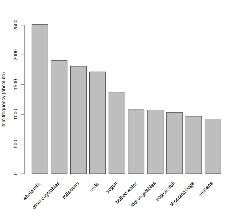
The top item purchased was whole milk with roughly 2,500 of the 9,836 transactions in the basket.

Look at the first five transactions

inspect(Groceries[1:5])

Modeling and evaluation

Throughout the modeling process, we will use the apriori algorithm, which is the appropriately named apriori() function in the arules package. The two main things that we will need to specify in the function is the dataset and parameters. As for the parameters, you will need to apply judgment when specifying the minimum support, confidence, and the minimum and/or maximum length of basket items in an itemset.

Using the item frequency plots, along with trial and error, let's set the minimum support at 1 in 1,000 transactions and minimum confidence at 90 percent. Additionally, let's establish the maximum number of items to be associated as four. The following is the code to create the object that we will call rules

rules <- apriori(Groceries, parameter = list(supp = 0.001, conf = 0.9, maxlen=4))

You will always have to pass the minimum required support and confidence.

• We set the minimum support to 0.001
• We set the minimum confidence of 0.9
• We then show the top 5 rules

Calling the object shows how many rules the algorithm produced.

There are a number of ways to examine the rules. The first thing that I recommend is to set the number of displayed digits to only two, with the options() function in base R. Then, sort and inspect the top five rules based on the lift that they provide, as follows:

options(digits = 2)
rules <- sort(rules, by = "lift", decreasing = TRUE)
inspect(rules[1:5])

The rule that provides the best overall lift is the purchase of liquor and red wine on the probability of purchasing bottled beer.

You can also sort by the support and confidence, so let's have a look at the first 5 rules by="confidence" in descending order, as follows:

rules <- sort(rules, by = "confidence", decreasing = TRUE)
inspect(rules[1:5])

You can see in the table that confidence for these transactions is 100 percent. Moving on to our specific study of beer, we can utilize a function in arules to develop cross tabulations - the crossTable() function - and then examine whatever suits our needs. The first step is to create a table with our dataset:

tab <- crossTable(Groceries)

With tab created, we can now examine the joint occurrences between the items.

As you might imagine, shoppers only selected liver loaf 50 times out of the 9,835 transactions. Additionally, of the 924 times, people gravitated toward sausage, 10 times they felt compelled to grab liver loaf. If you want to look at a specific example, you can either specify the row and column number or just spell that item out:

table["bottled beer","bottled beer"]

This tells us that there were 792 transactions of bottled bottled beer. Let's see what the joint occurrence between bottled beer and canned beer is:

table["bottled beer","canned beer"]

We can now move on and derive specific rules for bottled beer. We will again use the apriori() function, but this time, we will add a syntax around appearance. This means that we will specify in the syntax that we want the left-hand side to be items that increase the probability of a purchase of bottled beer, which will be on the right-hand side. In the following code, notice that I've adjusted the support and confidence numbers. Feel free to experiment with your own settings:

beer.rules <- apriori(data = Groceries, parameter = list(support
= 0.0015, confidence = 0.3), appearance = list(default = "lhs",
rhs = "bottled beer"))

We find ourselves with only 4 association rules. We have seen one of them already. Now let's bring in the other three rules in descending order by lift:

beer.rules <- sort(beer.rules, decreasing = TRUE, by = "lift")
inspect(beer.rules)

In all of the instances, the purchase of bottled beer is associated with booze, either liquor and/or red wine, which is no surprise to anyone. What is interesting is that white wine is not in the mix here. Let's take a closer look at this and compare the joint occurrences of bottled beer and types of wine:

tab["bottled beer", "red/blush wine"]
[1] 48

tab["red/blush wine", "red/blush wine"]
[1] 189

48/189
[1] 0.25

tab["white wine", "white wine"]
[1] 187

tab["bottled beer", "white wine"]
[1] 22

22/187
[1] 0.12

It's interesting that 25 percent of the time, when someone purchased red wine, they also purchased bottled beer. But with white wine, a joint purchase only happened in 12 percent of the instances. We certainly don't know why in this analysis, but this could potentially help us to determine how we should position our product in this grocery store.

Another thing before we move on is to look at a plot of the rules. This is done with the plot() function in the arulesViz package. There are many graphic options available. For this example, let's specify that we want a graph, showing lift, and the rules provided and shaded by confidence. The following syntax will provide this accordingly:

plot(beer.rules, method="graph", measure="lift", shading="confidence")

The following is the output of the preceding command:

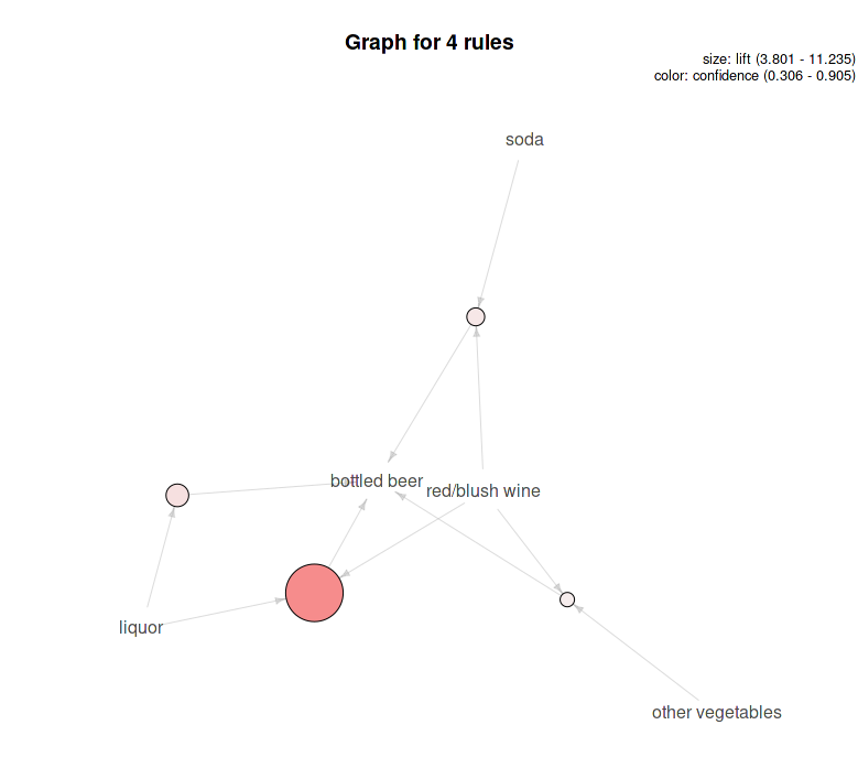
This graph shows that liquor/red wine provides the best lift and the highest level of confidence with both the size of the circle and its shading.

Find what factors influenced an event X

To find out what customers had purchased before buying Whole Milk. This will help you understand the patterns that led to the purchase of *whole milk.

rules <- apriori (data=Groceries, parameter=list (supp=0.001,conf = 0.08), 
appearance = list (default="lhs",rhs="whole milk"), control = list (verbose=F))

Find out what events were influenced by a given event

In this case: the Customers who bought Whole Milk also bought. In the equation, whole milk is in LHS (left hand side).

rules <- apriori (data=Groceries, parameter=list (supp=0.001,conf = 0.15,minlen=2), 
appearance = list (default="rhs",lhs="whole milk"), control = list (verbose=F))