Principal Component Analysis (PCA) in R Science 15.11.2016

Principal Component Analysis (PCA) is a dimensionality reduction technique that is widely used in data analysis. More concretely, PCA is used to reduce a large number of correlated variables into a smaller set of uncorrelated variables called principal components.

Introduction

In many datasets, particularly in the social sciences, you will see many variables highly correlated with each other. It may additionally suffer from high dimensionality or, as it is known, the curse of dimensionality. The goal then is to use PCA in order to create a smaller set of variables that capture most of the information from the original set of variables, thus simplifying the dataset and often leading to hidden insights. These new variables (principal components) are highly uncorrelated with each other.

Dimensionality reduction is a process of features extraction rather than a feature selection process. Feature extraction is a process of transforming the data in the high-dimensional space to a space of fewer dimensions.

Why do we need to reduce the dimension of the data? Well sometimes it's just difficult to do analysis on high dimensional data, especially on interpreting it. This is because there are dimensions that aren't significant which adds to our problem on the analysis. So in order to deal with this, we remove those nuisance dimension and deal with the significant one.

PCA is the process of finding the principal components. The first principal component in a dataset is the linear combination that captures the maximum variance in the data. A second component is created by selecting another linear combination that maximizes the variance with the constraint that its direction is perpendicular to the first component. The subsequent components (equal to the number of variables) would follow this same rule.

Modeling in R

There are many packages and functions that can apply PCA in R. In this post I will use the function prcomp() from the stats package.

There are several functions prcomp() and princomp() from the built-in R stats package.

• The function princomp() uses the spectral decomposition approach.
• The function prcomp() uses the singular value decomposition (SVD).

Function prcomp() performs a singular value decomposition directly on the data matrix this is slightly more accurate than doing an eigenvalue decomposition on the covariance matrix but conceptually equivalent. Therefore, prcomp() is the preferred function.

I will use the classical iris dataset for the demonstration. The data contain four continuous variables which corresponds to physical measures of flowers and a categorical variable describing the flowers' species.

# load and explore data 
data(iris)
head(iris, 3)

We will apply PCA to the four continuous variables and use the categorical variable to visualize the PCs later. PCA is sensitive to scale, so the data has been scaled with a log() transformation to the continuous variables. This is necessary if the input variables have very different variances, beside log transformation we can use scale() function. Also we set center and scale equal to TRUE in the call to prcomp() to standardize the variables prior to the application of PCA:

# log transform
log.ir = log(iris[, 1:4])
ir.species = iris[, 5]

Once you have standardised your variables, you can carry out a principal component analysis using the prcomp() function in R.

ir.pca = prcomp(log.ir, center = TRUE, scale. = TRUE)

The prcomp() function returns an object of class prcomp, which have some methods available. The print() method returns the standard deviation of each of the four PCs, and their rotation (or loadings), which are the coefficients of the linear combinations of the continuous variables. The standard deviations here are the square roots of the eigenvalues.

print(ir.pca)

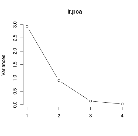
The plot() method returns a plot of the variances (y-axis) associated with the PCs (x-axis). The figure below is useful to decide how many PCs to retain for further analysis. In this simple case with only 4 PCs this is not a hard task and we can see that the first two PCs explain most of the variability in the data.

plot(ir.pca, type = "l")

By seeing the graph we could say that the first two principal components are able to explain great part of our data. However isn't there any less subjective way to choose our principal components? Yes, the easiest ways are by using two criteria: Kaiser-Guttman criterion and Broken Stick criterion. They are both based on the eigenvalues, which tell us how much a principal component is able to explain of our initial data set. To get our eigenvalues, just call:

ev = ir.pca$sdev^2

Now we can use the eigenvalues to contruct a very useful graph that can be help us to decide which princiapl components we need to choose. Copy and paste following evplot() function into R. I've slightly modify it to look more pretty. Original function here. Then, you can call evplot()

evplot = function(ev) {
  # Broken stick model (MacArthur 1957)
  n = length(ev)
  bsm = data.frame(j=seq(1:n), p=0)
  bsm$p[1] = 1/n
  for (i in 2:n) bsm$p[i] = bsm$p[i-1] + (1/(n + 1 - i))
  bsm$p = 100*bsm$p/n
  # Plot eigenvalues and % of variation for each axis
  op = par(mfrow=c(2,1),omi=c(0.1,0.3,0.1,0.1), mar=c(1, 1, 1, 1))
  barplot(ev, main="Eigenvalues", col="bisque", las=2)
  abline(h=mean(ev), col="red")
  legend("topright", "Average eigenvalue", lwd=1, col=2, bty="n")
  barplot(t(cbind(100*ev/sum(ev), bsm$p[n:1])), beside=TRUE, 
          main="% variation", col=c("bisque",2), las=2)
  legend("topright", c("% eigenvalue", "Broken stick model"), 
         pch=15, col=c("bisque",2), bty="n")
  par(op)
}

evplot(ev)

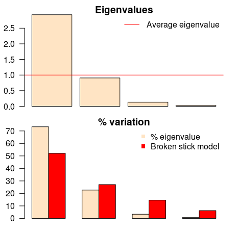
The first barplot tells us (according to Kaiser-Guttman criterion) that only the first principal component should be chosen (because its bar is above the red line). The same component should be chosen according to the other barplot (broken stick model), because it has the only bar above the red bar. Simple as that.

The summary() method describe the importance of the PCs. The first row describe again the standard deviation associated with each PC. The second row shows the proportion of the variance in the data explained by each component while the third row describe the cumulative proportion of explained variance. We can see there that the first two PCs accounts for more than 95% of the variance of the data.

summary(ir.pca)

We can use the predict() function if we observe new data and want to predict their PCs values. Just for illustration pretend the last two rows of the iris data has just arrived and we want to see what is their PCs values:

# predict PCs
predict(ir.pca, newdata=tail(log.ir, 2))

You might want to see how our initial variables contribute to two or three principal components, and how observations are explained by components. We can use a ggbiplot() for that. Note that choices is the argument defining which principal components will be used on the ggbiplot() (we will use the first two components).

library(devtools)
install_github("ggbiplot", "vqv")
library(ggbiplot)
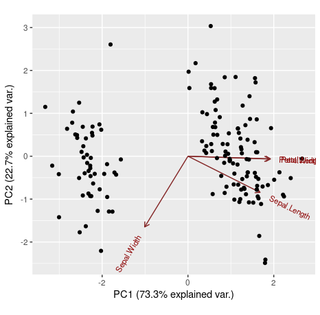
ggbiplot(ir.pca, choices=c(1,2), obs.scale = 1, var.scale = 1)

We can also use our fifth variable from the iris data set (the categorical variable iris[,5]) to define groups on the ggbiplot(). In that way, observations that belong to the same Iris' species will be grouped.

ggbiplot(ir.pca,choices=c(1,2), groups=iris[,5], obs.scale = 1, var.scale = 1, ellipse = TRUE)

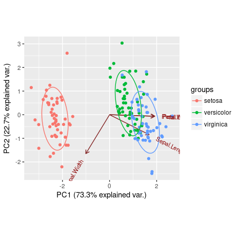
We can see that Petal.Length, Petal.Width and Sepal.Length are positively explained by the first principal component, while the Sepal.Width is negatively explained by it. Also, the second principal component was only able to negatively explain Sepal.Width and Sepal.Length.

So, advantages of Principal Component Analysis include:

• Reduces the time and storage space required.
• Remove multi-collinearity and improves the performance of the machine learning model.
• Makes it easier to visualize the data when reduced to very low dimensions such as 2D or 3D.