Of confidence intervals and example in R Science 05.04.2014

Introduction

A confidence interval (CI) is an interval estimate of a population parameter and is used to indicate the reliability of an estimate and can be interpreted as the range of values that would contain the true population value 95% of the time if the survey were repeated on multiple samples.

The "90%" in the confidence interval listed above represents a level of certainty about our estimate. If we were to repeatedly make new estimates using exactly the same procedure (by drawing a new sample, conducting new interviews, calculating new estimates and new confidence intervals), the confidence intervals would contain the average of all the estimates 90% of the time. We have therefore produced a single estimate in a way that, if repeated indefinitely, would result in 90% of the confidence intervals formed containing the true value.

Confidence intervals are one way to represent how "good" an estimate is; the larger a 90% confidence interval for a particular estimate, the more caution is required when using the estimate. Confidence intervals are an important reminder of the limitations of the estimates.

Practical example

Say you were interested in the mean weight of 10-year-old girls living in the United States. Since it would have been impractical to weigh all the 10-year-old girls in the United States, you took a sample of 16 and found that the mean weight was 90 pounds. This sample mean of 90 is a point estimate of the population mean. A point estimate by itself is of limited usefulness because it does not reveal the uncertainty associated with the estimate; you do not have a good sense of how far this sample mean may be from the population mean. For example, can you be confident that the population mean is within 5 pounds of 90? You simply do not know.

Confidence intervals provide more information than point estimates. Confidence intervals for means are intervals constructed using a procedure (presented in the next section) that will contain the population mean a specified proportion of the time, typically either 95% or 99% of the time. These intervals are referred to as 95% and 99% confidence intervals respectively. An example of a 95% confidence interval is shown below:

72.85 < μ < 107.15

There is good reason to believe that the population mean lies between these two bounds of 72.85 and 107.15 since 95% of the time confidence intervals contain the true mean.

If repeated samples were taken and the 95% confidence interval computed for each sample, 95% of the intervals would contain the population mean. Naturally, 5% of the intervals would not contain the population mean.

Source.

Simulation in R

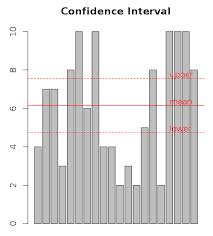
Let's simulate confidence interval in R and plot the result.

Say you have a sample from a population. Given that sample, you want to determine a confidence interval for the population’s mean.

We'll apply the t.test function to your sample x t.test(x). The output includes a confidence interval at the 95% confidence level. To see intervals at other levels, use the conf.level argument.

x = sample(10, 20, replace=T)
# [1]  1  3  5  3  9  6  2  9  8  6  7  4 10  8  5  4  7  2  7  5

t.test(x)
#   One Sample t-test
# data:  x
# t = 9.6021, df = 19, p-value = 1.008e-08
# alternative hypothesis: true mean is not equal to 0
# 95 percent confidence interval:
# 4.340241 6.759759
# sample estimates:
# mean of x 
#     5.55

lower = t.test(x)$conf.int[1]
upper = t.test(x)$conf.int[2]

amount = length(x)

barplot(x, main="Confidence Interval")

# plot mean
abline(h=mean(x), lty=1, col="red")
text(amount, mean(x), "mean", col="red", adj=c(0, -0.2))

# plot upper
abline(h=upper, lty=2, col="red")
text(amount, upper, "upper", col="red", adj=c(0, -0.2))

# plot lower
abline(h=lower, lty=2, col="red")
text(amount, lower, "lower", col="red", adj=c(0, -0.2))

Useful links

• How to Calculate Confidence Interval