How-to simulate genetic algorithms in R Science 10.04.2014

Introduction

Genetic Algorithms are a family of computational models inspired by evolution. They are used for a number of different application areas. An example of this would be multidimensional optimization problems in which the character string of the chromosome can be used to encode the values for the different parameters being optimized.

Genetic algorithms are good at finding the better locations on a global scale. GAs have been successfully applied to solve optimization problems, both for continuous (whether differentiable or not) and discrete functions.

Main purpose of GAs are:

• In computer science and AI, as a process of search through the space of possible solutions. The set of possible solutions defines the search space (also called state space) for a given problem. Solutions or partial solutions are viewed as points in the search space.
• In engineering and mathematics, as a process of optimization. The problems are first formulated as mathematical models expressed in terms of functions and then to find a solution, discover the parameters that optimize the model or the function components that provide optimal system performance.

Optimization is a process that finds a best, or optimal, solution for a problem. The Optimization problems are centered around three factors :

1. An objective function which is to be minimized or maximized.
2. A set of unknowns or variables that affect the objective function.
3. A set of constraints that allow the unknowns to take on certain values but exclude others.

An optimization problem is defined as: Finding values of the variables that minimize or maximize the objective function while satisfying the constrains.

There are at least three situations where genetic algorithms are useful:

• The objective function is not smooth (i.e., not differentiable).
• There are multiple local optima.
• There is a large number of parameters (the meaning of “large” keeps changing).

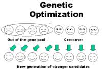
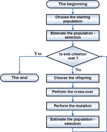
The typical algorithm selects two "parents" from the population, and commingles their "genes" to get a new solution. This new solution may or may not enter the population depending on how good its objective is.

GAs are based on an analogy with the genetic structure and behaviour of chromosomes within a population of individuals using the following foundations:

A GAs consist of three things:

1. A gene. The gene is typically a binary number, each bit in the binary number controls various parts of feature in your model.
2. A fitness function. A gene is quantified as a good or bad gene using a fitness function.
3. Methods to breed/mate genes. Crossover.

The most commonly used methods of selecting chromosomes for parents to crossover are :

• Roulette wheel selection.
• Rank selection.
• Boltzmann selection.
• Steady state selection.
• Tournament selection.

Modeling GAs in R

The following is example from http://fishyoperations.com/. For demonstration it explains the Knapsack problem.

Task description: you are going to spend a month in the wilderness. You’re taking a backpack with you, however, the maximum weight it can carry is 20 kilograms. You have a number of survival items available, each with its own number of "survival points". You’re objective is to maximize the number of survival points.

ITEM	SURVIVALPOINTS	WEIGHT
pocketknife	10	1
beans	20	5
potatoes	15	10
unions	2	1
sleeping bag	30	7
rope	10	5
compass	30	1

In R I have used the package genalg to set-up the model.

First of all, let's install genalg.

install.packages("genalg")

Let's define the dataset and weight constraint.

library(genalg)

dataset = data.frame(item = c("pocketknife", "beans", "potatoes", "unions", 
"sleeping bag", "rope", "compass"), 
survivalpoints = c(10, 20, 15, 2, 30, 10, 30), weight = c(1, 5, 10, 1, 7, 5, 1))
weightlimit = 20

Before creating the model we have to set-up an evaluation function. The evaluation function will evaluate the different individuals (chromosomes) of the population on the value of their gene configuration.

An individual can for example have the following gene configuration: 1001100.

Each number in this binary string represents whether or not to take an item with you. A value of 1 refers to putting the specific item in the knapsack while a 0 refers to leave the item at home. Given the example gene configuration we would take the following items.

chromosome = c(1, 0, 0, 1, 1, 0, 0)
dataset[chromosome == 1, ]
##           item survivalpoints weight
## 1  pocketknife             10      1
## 4       unions              2      1
## 5 sleeping bag             30      7

We can check to what amount of surivival points this configuration sums up.

cat(chromosome %*% dataset$survivalpoints)
## 42

Above we gave a value to the gene configuration of a given chromosome. This is exactly what the evaluation function does.

The genalg algorithm tries to optimize towards the minimum value. Therefore, the value is calculated as above and multiplied with -1. A configuration which leads to exceeding the weight constraint returns a value of 0 (a higher value can also be given).

We define the evaluation function as follows.

evalFunc = function(x) {
    current_solution_survivalpoints = x %*% dataset$survivalpoints
    current_solution_weight = x %*% dataset$weight

    if (current_solution_weight > weightlimit) 
        return(0) 
    else 
        return(-current_solution_survivalpoints)
}

Next, we choose the number of iterations, design and run the model.

iter = 100
GAmodel = rbga.bin(size = 7, popSize = 200, iters = iter, mutationChance = 0.01, elitism = T, evalFunc = evalFunc)
cat(summary.rbga(GAmodel))
## GA Settings
##   Type                  = binary chromosome
##   Population size       = 200
##   Number of Generations = 100
##   Elitism               = TRUE
##   Mutation Chance       = 0.01
## 
## Search Domain
##   Var 1 = [,]
##   Var 0 = [,]
## 
## GA Results
##   Best Solution : 1 1 0 1 1 1 1 

The best solution is found to be 1111101. This leads us to take the following items with us on our trip into the wild.

solution = c(1, 1, 1, 1, 1, 0, 1)
dataset[solution == 1, ]
##           item survivalpoints weight
## 1  pocketknife             10      1
## 2        beans             20      5
## 3     potatoes             15     10
## 4       unions              2      1
## 5 sleeping bag             30      7
## 7      compass             30      1

This in turn gives us the total number of survival points.

# solution vs available
cat(paste(solution %*% dataset$survivalpoints, "/", sum(dataset$survivalpoints)))
## 107 / 117

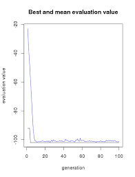
Let's visualize how the model evolves.

plot(GAmodel)

Vocabulary

• Chromosomes are strings of DNA (DeoxyriboNucleic Acid) and serve as a model for the whole organism.
• Genes are block of chromosomes. Each gene encodes a particular protein that represents a trait (feature), e.g., color of eyes.
• Alleles are possible settings for a trait (e.g. blue, brown)
• Locus is the position of gene in the chromosome.
• Genome is complete set of genetic material (all chromosomes).
• Genotype is particular set of genes in a genome.
• Phenotype is physical expression of the genotype (the organism itself after birth). Its physical and mental characteristics, such as eye color, intelligence etc.
• Crossover. When two organisms mate they share their genes; the resultant offspring may end up having half the genes from one parent and half from the other. This process is called recombination (cross over).
• Mutation. The new created offspring can then be mutated. Mutation means, that the elements of DNA are a bit changed. This changes are mainly caused by errors in copying genes from parents.
• Survival. The fitness of an organism is measured by success of the organism in its life.

Useful links

• Genetic algorithm by Tom V. Mathew
• Artificial Intelligence
• GA: A Package for Genetic Algorithms in R
• Genetic algorithms (in Russian)