R as instrument for modeling Science 23.03.2014

R is a free software programming language and software environment for statistical computing and graphics. The R language is widely used among statisticians and data miners for developing statistical software and data analysis (source). More about R popularity you can see here.

I am going to install R language and RStudio as IDE.

# arch
yaourt -S r rstudio-desktop-bin

# ubuntu 
sudo apt-get install r-base

The latest version of RStudio for Ubuntu can be found here. Download it and install with next command

sudo dpkg -i rstudio-0.98.501-amd64.deb

Data types

R has such data types: numbers, strings, logical, factor, vector, list, matrix, data frame. Almost all data structures are built upon these five types. Hadley Wickham, in his book Advanced R, provided an easy-to-comprehend segregation of these five data structures

# number
n <- 7

# string 
s <- "string"

# concatenate two strings
s1 <- "Hello, "; s2 <- "world!"
paste(s1, s2)

# format string 
sprintf("Hello, %s. It's %d am.", "user", 10)

# logical
l <- TRUE

A vector is a sequence of data elements of the same basic type. A vector can contain any number of elements. However, all the elements must be of the same type; for instance, a vector cannot contain both numbers and text.

v1 <- c(1, 2, 3, 4, 5)
[1] 1 2 3 4 5

# sequence
v2 <- seq(1,5)
[1] 1 2 3 4 5

v3 <- 1:5
[1] 1 2 3 4 5

v3 <- 5:1
[1] 5 4 3 2 1

# sequence with step
v4 <- seq(from = 1, to = 5, by = 0.5)
[1] 1.0 1.5 2.0 2.5 3.0 3.5 4.0 4.5 5.0

# sequence with boundaries, increment is calculated automaticaly 
v5 <- seq(from=1, to=5, length.out=6)
[1] 1.0 1.8 2.6 3.4 4.2 5.0

# a series of repeated values
v6 <- rep(1, times=5)

v7 <- rep(1:3, times=3)
[1] 1 2 3 1 2 3 1 2 3

# repeat 1 time 2 and 3 time 4
v8 <- rep(c(2,4), c(1,3))
[1] 2 4 4 4

# the number of members in a vector
length(v1)

Indexing vector

v1 <- c(1, 2, 3, 4, 5)

v1[3]
[1] 3

# range of items
v1[2:4]
[1] 2 3 4

# items by order
v1[c(1,3,5)]
[1] 1 3 5

# exclude 2nd and 4th items
v1[-c(2,4)]

# logical vector indicating whether each item should be included
v1[c(TRUE, TRUE, FALSE, FALSE, TRUE)]

# all items greater than 3 
v1[v1 > 3]
[1] 4 5

# get indexes of all items which values is greater than 3
which(v1 > 3)
[1] 4 5

# all values that is greater 1 and less 5
> v1[v1 > 1 & v1 < 5]
[1] 2 3 4

# indexing by name
names(v1) <- c("one", "two", "three", "four", "five")
v1["one"]
one 
  1

v1[c("one", "three")]
  one three 
    1     3

Vector arithmetic

v1 <- 1:5
v2 <- 5:10

# multiple each member by 5
v1 * 5

# the sum would be a vector whose members are the sum of the corresponding members from v1 and v2
v3 <- v1 + v2

Sort vector

sort(v1, decreasing=TRUE)
 five  four three   two   one 
    5     4     3     2     1

A matrix is a collection of data elements, of the same basic type, arranged in a two-dimensional rectangular layout.

Create matrix with 4 rows and 4 columns (4x4).

m <- matrix(seq(1, 16), nrow = 4, ncol = 4)

# fill matrix by rows
m <- matrix(seq(1, 16), nrow = 4, ncol = 4, byrow = TRUE)

# create matrix from vector
m <- 1:16
dim(m) <- c(4,4)

Matrix indexing

# element at 1st row, 2nd column
m[1, 2]

# the 3rd row
m[3,]

# the 3rd column
m[,3]

# the 3rd and 4th columns
m[, c(3,4)]

Matrix arithmetic

# multiple 1st and 4th columns
m[, 1] * m[, 4]

# transpose matrix
t(m)

A list is used for storing an ordered set of values. However, unlike a vector that requires all elements to be the same type, a list allows different types of values to be collected. When a list is constructed, you have the option of providing names (fullname), for each value in the sequence of items.

# create three vectors
v1 <- c("a", "b", "c")
v2 <- seq(1, 5)
v3 <- c(FALSE, TRUE, TRUE, FALSE)

# combine three vectors to list with names 
l <- list(Text=v1, Number=v2, Logic=v3)

# indexing 1st member
l[[1]]
l$Text

A data frame is used for storing data tables. It is a list of vectors of equal length. For example, the following variable tbl is a data frame containing three vectors car, year, owner.

car <- c("Ford", "BMW", "Audio")
year <- c(1972, 1976, 1983)
owner <- c("John", "Lisa", "Lisa")

tbl <- data.frame(Car=car, Year=year, Owner=owner, stringsAsFactors=FALSE)

# display the structure
str(tbl)

# indexing by column
tbl$Car

# get 3rd item from Year column
tbl$Year[3]

# extract several columns from a data frame
tbl[c("Year", "Owner")]

# extract the value in the 1st row and 2nd column
tbl[1, 2]

# get range from Year column
tbl$Year[1:3]

# get range from Year column where year is biger than 1972
tbl$Year[tbl$Year > 1972]

# get all cars which belongs to Lisa
tbl$Car[tbl$Owner == "Lisa"]

# lookup
# first 3 rows
head(tbl, n=3)

# last 3 rows
tail(tbl, n=3)

Import data frame from file

# from CSV file
tbl <- read.csv(file="table.csv", header=TRUE, sep=",");
names(tbl)

# from Excel file
library(gdata)
tbl <- read.xls("table.xls")

Plot data

There are many external packages for charts.

Following are internal abilities of R.

# random sequence for plot
v <- sample(1:10, 15, replace=TRUE)

Strip chart plots the data in order along a line with each data point represented as a box.

stripchart(v)

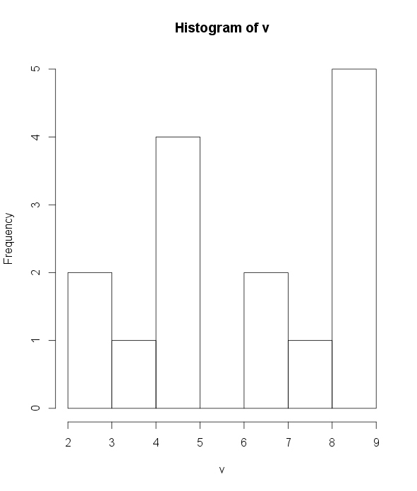
Histogram plots the frequencies that data appears within certain ranges.

hist(v, help="Distribution of v", xlab="v")

A boxplot provides a graphical view of the median, quartiles, maximum, and minimum of a data set.

boxplot(v)

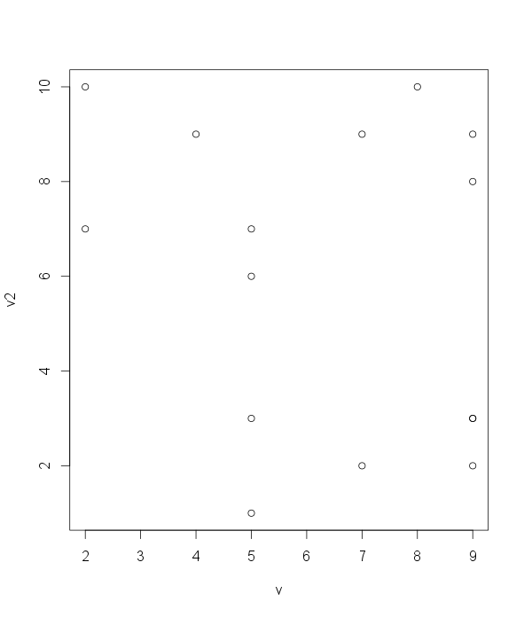
A scatter plot provides a graphical view of the relationship between two sets of numbers.

v2 < sample(1:10, 15, replace=TRUE)
plot(v, v2)

Statistics with R

The following commands can be used to get the mean, median, quantiles, minimum, maximum, variance, and standard deviation of a set of numbers:

# random sequence
v <- sample(1:10, 15, replace=TRUE)

mean(v)

median(v)

# quantiles
quantile(v)

# minimum
min(v)

# maximum
max(v)

# variance
var(v)

# standard deviation
sd(v)

# filter missing values
append(v, NA)
mean(v, na.rm=TRUE)
sd(v, na.rm=TRUE)

Finally, the summary command will print out the min, max, mean, median, and quantiles:

summary(v)

Min. 1st Qu.  Median    Mean 3rd Qu.    Max. 
1.0     5.0     8.0     6.8    10.0    10.0

The cor and cov functions can calculate the correlation and covariance, respectively, between two vectors:

# random sequence
v1 <- sample(1:10, 15, replace=TRUE)
v2 <- sample(1:10, 15, replace=TRUE)

cor(v1, v2)

cov(v1, v2)

The correlation between two variables is a number that indicates how closely their relationship follows a straight line. Without additional qualification, correlation typically refers to Pearson's correlation coefficient, which was developed by the 20th century mathematician Karl Pearson. The correlation ranges between -1 and +1. The extreme values indicate a perfectly linear relationship, while a correlation close to zero indicates the absence of a linear relationship.

Covariance is a measure of the linear relationship between two continuous variables. Covariance is scale dependent, meaning that the value depends on the units of measurements used for the variables. For this reason, it is difficult to directly interpret the covariance value. The higher the absolute covariance between two variables, the greater the association. Positive values indicate positive association and negative values indicate negative association.

Import/Export data

# save variables to file
save(v, v1, v2, file="myvar.RData")

# load variables from file
load("myvar.RData")

# save data frame to CSV
write.csv(df, file="df.csv")

# load data frame from CSV
df <- read.csv("df.csv", stringsAsFactors = FALSE, header = FALSE)

Also, we can import data from SQL databases (PostgreSQL, MySQL, and so on) with help of RODBC package.

# install and load library
install.packages("RODBC")
library(RODBC)

# create connection
mydb <- odbcConnect("DSN", uid="username", pwd="password")

# create query and execute it
query <- "select * from table where status = 1"
df <- sqlQuery(channel=mydb, query=query, stringsAsFactors=FALSE)

# close connection
odbcClose(mydb)

Packages

To install package

install.packages("package name")

To update packages

update.packages()

To see which packages are already installed on the computer, enter

installed.packages()

Help

Use help to display the documentation for the function:

help(functionname)
# or 
?(function)

Use args for a quick reminder of the function arguments:

args(functionname)

Use example to see examples of using the function:

example(functionname)

Useful links

• CRAN Task Views
• RSeek
• RTutorial