Getting Started with Time Series in R

Getting Started with Time Series in R Science 17.05.2016

Introduction

Time series is an ordered sequence of values of a variable at equally spaced time intervals. Ordering is very important because there is dependency and changing the order could change the meaning of the data. The usage of time series models is twofold:

Obtain an understanding of the underlying forces and structure that produced the observed data.
Fit a model and proceed to forecasting, monitoring or even feedback and feedforward control.

So, a time series is a collection of observations of well-defined data items obtained through repeated measurements over time. For example, measuring the value of retail sales each month of the year would comprise a time series. This is because sales revenue is well defined, and consistently measured at equally spaced intervals. Another example is the amount of rainfall in a region at different months of the year. Time series analysis is used for many applications such as: economic forecasting, sales forecasting, budgetary analysis, stock market analysis, process and quality control, utility studies, etc.

Data collected irregularly or only once are not time series.

An observed time series can be decomposed into three components: the trend (long term direction), the seasonal (systematic, calendar related movements) and the irregular (unsystematic, short term fluctuations).

Some important questions to first consider when first looking at a time series are:

Is there a trend, meaning that, on average, the measurements tend to increase (or decrease) over time?
Is there seasonality, meaning that there is a regularly repeating pattern of highs and lows related to calendar time such as seasons, quarters, months, days of the week, and so on?
Are their outliers? In regression, outliers are far away from your line. With time series data, your outliers are far away from your other data.
Is there a long-run cycle or period unrelated to seasonality factors?
Is there constant varianceover time, or is the variance non-constant?
Are there any abrupt changes to either the level of the series or the variance?

One simple method of describing a series is that of classical decomposition. The notion is that the series can be decomposed into four elements:

Trend (T_t) - long term movements in the mean;
Seasonal effects (S_t) - cyclical fluctuations related to the calendar;
Irregular component (or residuals) (I_t) - other random or systematic fluctuations.

The idea is to create separate models for these three elements and then combine them, either additively

$X_t=T_t+S_t+I_t$

or multiplicatively

$X_t=T_t \cdot S_t \cdot I_t$

So, decomposition models are typically additive or multiplicative, but can also take other forms such as pseudo-additive.

To choose an appropriate decomposition model, the time series analyst will examine a graph of the original series and try a range of models, selecting the one which yields the most stable seasonal component.

In some time series, the amplitude of both the seasonal and irregular variations do not change as the level of the trend rises or falls. In such cases, an additive model is appropriate.
In many time series, the amplitude of both the seasonal and irregular variations increase as the level of the trend rises.In this situation, a multiplicative model is usually appropriate.
The multiplicative model cannot be used when the original time series contains very small or zero values. This is because it is not possible to divide a number by zero. In these cases, a pseudo additive model combining the elements of both the additive and multiplicative models is used. This model assumes that seasonal and irregular variations are both dependent on the level of the trend but independent of each other.

Modeling in R

R has extensive facilities for analyzing time series data.

The first thing that you will want to do to analyse your time series data will be to read it into R, and to plot the time series. You can read data into R using the scan() function, which assumes that your data for successive time points is in a simple text file with one column.

# read from url 
petrol = scan("http://url/petrol.dat")

# or from vector
petrol = c(
47,34,49,41,13,35,53,56,16,43,69,59, 
60,43,67,50,56,42,50,65,68,43,65,34, 
59,86,55,68,51,33,49,67,77,81,67,71
)

Once you have read the time series data into R, the next step is to store the data in a time series object in R, so that you can use R’s many functions for analysing time series data. To store the data in a time series object, we use the ts() function in R.

petrol.ts = ts(petrol, start=c(2014,1), frequency=12)

Sometimes the time series data that you have been collected at regular intervals that were less than one year, for example, monthly or quarterly. In this case, you can specify the number of times that data was collected per year by using the frequency parameter in the ts() function. For monthly time series data, you set frequency=12, while for quarterly time series data, you set frequency=4.

You can also specify the first year that the data was collected, and the first interval in that year by using the start parameter in the ts() function, so start specifies the start time for the first observation in time series. For example, if the first data point corresponds to the second quarter of 2016, you would set start=c(2016,1).

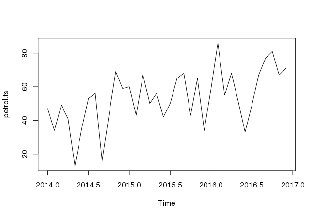
Once you have read a time series into R, the next step is usually to make a plot of the time series data, which you can do with the plot.ts() function in R.

plot.ts(petrol.ts)

We can plot time series for specific period

plot(petrol.ts, type="l", xlim=c(2014,2015))

Decomposing a time series means separating it into its components, which are usually a trend component and an irregular component, and if it is a seasonal time series, a seasonal component.

Decomposing Non-Seasonal Data

A non-seasonal time series consists of a trend component and an irregular component. To estimate the trend component of a non-seasonal time series that can be described using an additive model, it is common to use a smoothing method, such as calculating the simple moving average of the time series. The SMA() function in the TTR R package can be used to smooth time series data using a simple moving average.

Decomposing Seasonal Data

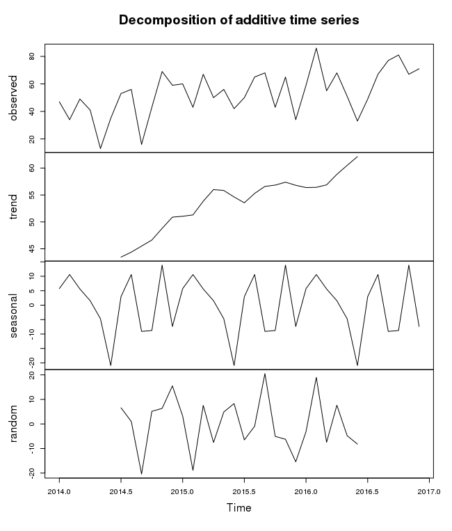
A seasonal time series consists of a trend component, a seasonal component and an irregular component. To estimate the trend component and seasonal component of a seasonal time series that can be described using an additive model, we can use the decompose() function in R. This function estimates the trend, seasonal, and irregular components of a time series that can be described using an additive model. The function decompose() returns a list object as its result, where the estimates of the seasonal component, trend component and irregular component are stored in named elements of that list objects, called seasonal, trend, and random respectively.

To estimate the trend, seasonal and irregular components of our petrol time series, we type:

petrol.componets = decompose(petrol.ts)

The estimated values of the seasonal, trend and irregular components are now stored in variables petrol.componets$seasonal, petrol.componets$trend and petrol.componets$random.

We can plot the estimated trend, seasonal, and irregular components of the time series by using the plot() function, for example:

plot(petrol.componets)

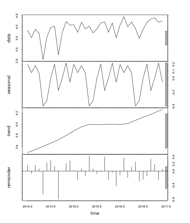
Another possibility for evaluating the trend of a time series is to use nonparametric regression techniques (which in fact can be seen as a special case of linear filters). The function stl() performs a seasonal decomposition of a given time series X_t by determining the trend T_t using loess regression and then calculating the seasonal component S_t (and the residuals E_t) from the differences X_t − T_t.

Performing the seasonal decomposition for the time series petrol is done using the following commands:

plot(stl(log(petrol.ts), s.window="periodic"))

Exponential Smoothing and Prediction of Time Series

A natural estimate for predicting the next value of a given time series x_t at the period t is to take weighted sums of past observations.

Exponential smoothing in its basic form (the term exponential comes from the fact that the weights decay exponentially) should only be used for time series with no systematic trend and/or seasonal components. It has been generalized to the Holt–Winters–procedure in order to deal with time series containg trend and seasonal variation. In this case, three smoothing parameters are required, namely alfa (for the level), beta (for the trend) and gamma (for the seasonal variation).

The R contains the function HoltWinters(x, alpha, beta, gamma), which lets one perform the Holt–Winters procedure on a time series x. One can specify the three smoothing parameters with the options alpha, beta and gamma. Particular components can be excluded by setting the value of the corresponding parameter to zero, e.g. one can exclude the seasonal component by using gamma=0. In case one does not specify smoothing parameters, these are determined automatically.

HoltWinters(petrol)

This performs the Holt–Winters procedure on the petrol dataset. It displays a list with smoothing parameters.

R offers the function predict(), which is a generic function for predictions from various models. In order to use predict(), one has to save the fit of a model to an object, e.g.:

petrol.hw = HoltWinters(petrol.ts)
predict(petrol.hw, n.ahead=12)

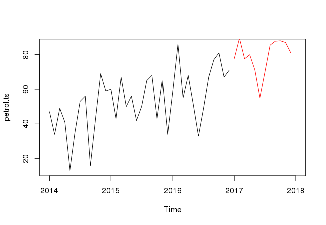
In this case, we have saved the fit from the Holt–Winters procedure on petrol as petrol.hw and got the predicted values for the next 12 periods.

The following commands can be used to create a graph with the predictions for the next 1 years (i.e. 12 months):

plot(petrol.ts, xlim=c(2014, 2018))
lines(predict(petrol.hw, n.ahead=12), col=2)

Autocorrelation functions

A first step in analyzing time series is to examine the autocorrelations (ACF) and partial autocorrelations (PACF).

One important property of a time series is the autocorrelation function. Just as correlation measures the extent of a linear relationship between two variables, autocorrelation measures the linear relationship between lagged values of a time series. Autocorrelation refers to the correlation of a time series with its own past and future values. Autocorrelation is also sometimes called lagged correlation or serial correlation, which refers to the correlation between members of a series of numbers arranged in time. Positive autocorrelation might be considered a specific form of persistence, a tendency for a system to remain in the same state from one observation to the next. For example, the likelihood of tomorrow being rainy is greater if today is rainy than if today is dry.

R provides the functions acf() and pacf() for computing and plotting of ACF and PACF.

Check set of autocorrelation coefficients

acf(petrol.ts, plot=FALSE)

The autocorrelation coefficients are normally plotted to form the autocorrelation function or ACF. The plot is also known as a correlogram.

acf(petrol.ts)

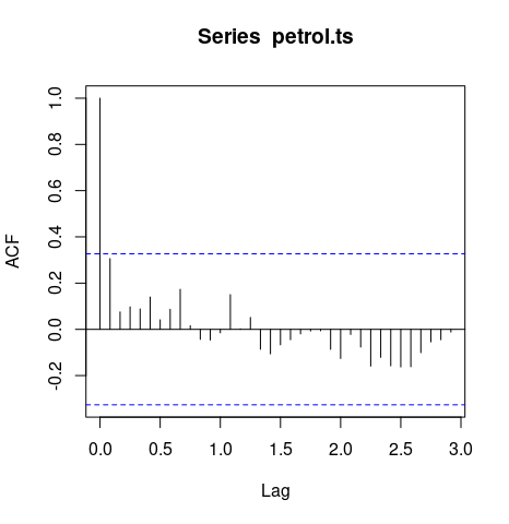
The ACF will first test whether adjacent observations are autocorrelated, that is, whether there is correlation between observations #1 and #2, #2 and #3, #3 and #4, etc. This is known as lag one autocorrelation, since one of the pair of tested observations lags the other by one period or sample. Similarly, it will test at other lags. For instance, the autocorrelation at lag four tests whether observations #1 and #5, #2 and #6, ...,#19 and #23, etc. are correlated. In general, we should test for autocorrelation at lags one to lag n/4, where n is the total number of observations in the analysis.

Autocorrelation plots are a commonly-used tool for checking randomness in a data set. This randomness is ascertained by computing autocorrelations for data values at varying time lags. If random, such autocorrelations should be near zero for any and all time-lag separations. If non-random, then one or more of the autocorrelations will be significantly non-zero.

Time series that show no autocorrelation are called white noise. For white noise series, we expect each autocorrelation to be close to zero.

Useful links

Getting Started with Time Series in R Science 17.05.2016

Quote

Categories

Archive ↓